Chapter 8 Variability and Waiting Time Problems A Call Center - - PDF document

2015/3/29 1

Chapter 8 Variability and Waiting Time Problems



A Call Center Example



Arrival Process and Service Variability



Predicting Waiting Times



Waiting Line Management

3

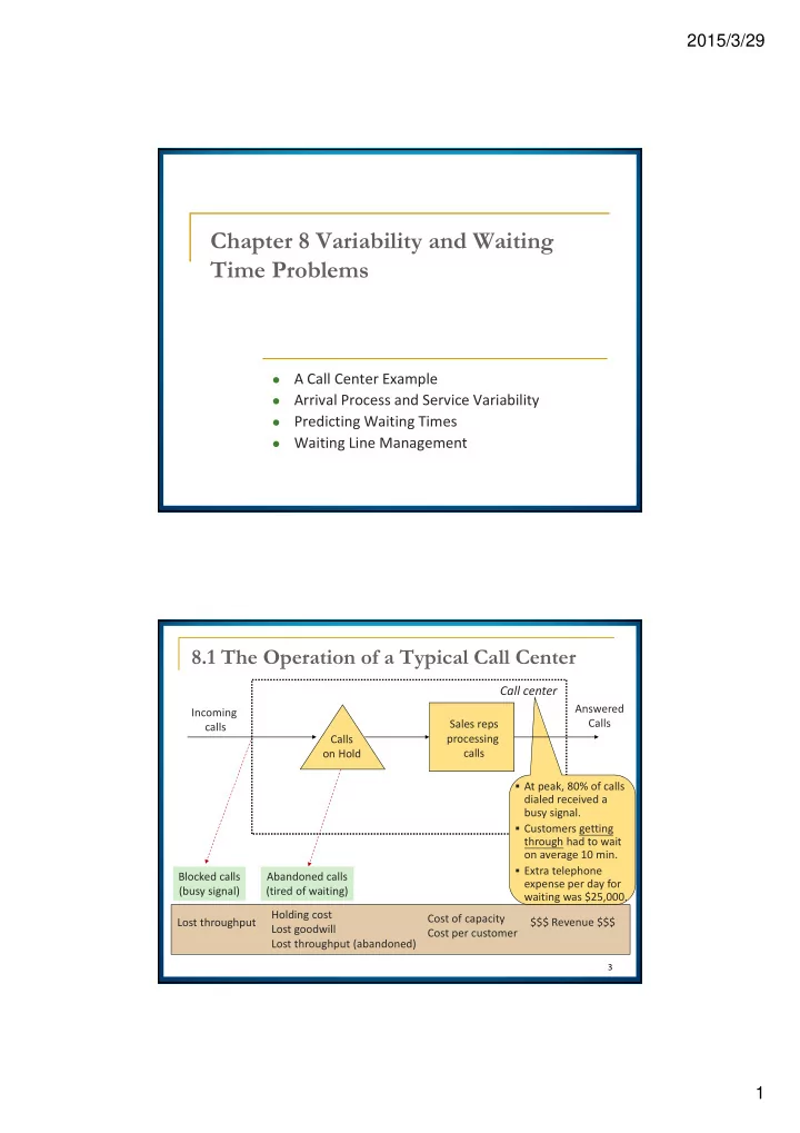
Blocked calls (busy signal) Abandoned calls (tired of waiting) Calls

• n Hold

Sales reps processing calls Answered Calls Incoming calls

Call center

Lost throughput Holding cost Lost goodwill Lost throughput (abandoned) $$$ Revenue $$$ Cost of capacity Cost per customer

• At peak, 80% of calls

dialed received a busy signal.

• Customers getting

through had to wait

• n average 10 min.
• Extra telephone

expense per day for waiting was $25,000.

8.1 The Operation of a Typical Call Center

2015/3/29 2

4

7:00 7:10 7:20 7:30 7:40 7:50 8:00

Patient Arrival Time Service Time

1 2 3 4 5 6 7 8 9 10 11 12 5 10 15 20 25 30 35 40 45 50 55 4 4 4 4 4 4 4 4 4 4 4 4

A “Perfect or Somewhat Odd” Call Center

5 Patient Arrival Time Service Time

1 2 3 4 5 6 7 8 9 10 11 12 7 9 12 18 22 25 30 36 45 51 55 5 6 7 6 5 2 4 3 4 2 2 3 Time 7:10 7:20 7:30 7:40 7:50 8:00 7:00

Patient 1 Patient 3 Patient 5 Patient 7 Patient 9 Patient 11 Patient 2 Patient 4 Patient 6 Patient 8 Patient 10 Patient 12 1 2 3 2 min. 3 min. 4 min. 5 min. 6 min. 7 min.

Service times Number of cases

A More Realistic Service Process

2015/3/29 3

6

7:00 7:10 7:20 7:30 7:40 7:50

Inventory (Patients at lab)

5 4 3 2 1

8:00

7:00 7:10 7:20 7:30 7:40 7:50 8:00

Wait time Service time Patient Arrival Time Service Time

1 2 3 4 5 6 7 8 9 10 11 12 7 9 12 18 22 25 30 36 45 51 55 5 6 7 6 5 2 4 3 4 2 2 3

Variability Leads to Waiting Time

7

Most customers have to wait, although,

• n average, there is plenty of capacity

in the call center. The call canter is unable to provide consistent service quality. If customer abandon calls after long waits, the call center loses customer goodwill and revenue.

Observations

2015/3/29 4

8

Input

• Unpredicted

Volume swings

• Random arrivals

(randomness is the rule, not the exception)

• Incoming quality
• Product Mix

Resources

• Breakdowns / Maintenance
• Operator absence
• Set‐up times

Tasks

• Inherent variation
• Lack of SOPs
• Quality (scrap / rework)

Routes

• Variable routing
• Dedicated machines

Buffer Processing

8.2 Variability: Where does it come from?

9

Ignoring Variability Leads to Problems

A: You cannot inventory services — Capacity can never run ahead of demand. Random arrivals and varying demands are common in services. In the presence of variability,

• ne cannot estimate the process

performance based on averages. Q: Why does variability not average out over time?

2015/3/29 5

10

8.3 Analyzing an Arrival Process

Call Arrival Time, ATi

1 2 3 4 5 6 7 6:00:29 6:00:52 6:02:16 6:02:50 6:05:14 6:05:50 6:06:28

Interarrival Time IAi=ATi+1 ‐ATi

00:23 01:24 00:34 02:24 00:36 00:38 Time 6:01 6:02 6:03 6:04 6:05 6:06 6:00

Call 1 Call 2 Call 3 Call 4 Call 5 Call 6 Call 7 IA1 IA2 IA3 IA4 IA5 IA6

Mean Deviation Standard Variation

• f

t Coefficien 

11

Seasonality over the Course of a Day

20 40 60 80 100 120 140 160 0:15 2:00 3:45 5:30 7:15 9:00 10:45 12:30 14:15 16:00 17:45 19:30 21:15 23:00

per 15 minutes

20 40 60 80 100 120 140 160 0:15 2:00 3:45 5:30 7:15 9:00 10:45 12:30 14:15 16:00 17:45 19:30 21:15 23:00

Time

• no. of customers

An arrival process is not stationary if the average number of arrivals in any given time interval is not fixed over the entire time period.

2015/3/29 6

12

Exponential Distribution

10 20 30 40 50 60 70 80 90 100

Number of calls with given duration t Duration t

Customers arriving independently from each other follow exponential inter‐arrival times.  Random (Poisson) arrivals

a t

e a t f



 1 ) ( a = average inter‐arrival time

13

How to Analyze a Demand/Arrival Process

Stationary Arrivals?

YES NO

Break arrival process up into smaller time intervals

YES

Random Arrivals?

NO

• Compute a: average interarrival time
• CVa=1
• All results of chapters 8 and 9 apply
• Compute a: average interarrival time
• CVa= St.dev. of interarrival times/a
• All results of chapter 8 apply
• Results of chapter 9 do not apply, require

simulation or more advanced tools

time al interarriv Average time al interarriv

• f

deviation Standard CV mean  

a

a

2015/3/29 7

14

8.4 Service Times in Call Center

800 600 400 200

• Std. Dev = 141.46

Mean = 127.2 N = 2061.00

Call durations [seconds] Frequency

ime activity t Average ime activity t

• f

deviation Standard CV mean  

p

p

15

8.5 Predicting Average Waiting Time: One Server

Inflow Outflow Inventory waiting Iq Entry to system Departure Begin Service Waiting Time Tq Service Time p Flow Time T=Tq+p Inventory in service Ip

2015/3/29 8

16

Average flow time T Utilization 100%

Increasing Variability

Service time factor Utilization factor Variability factor

                   2 1 Time Activity queue in

2 2 p a

CV CV n utilizatio n utilizatio Time

The Waiting Time Formula

% 100 / 1 / 1 capacity rate flow n utilizatio     a p p a

17

Reducing average waiting time does not guarantee customer satisfaction. A small percentage of customers may experience long waits and complain bitterly. Solution: service guarantee and/or service recovery

2015/3/29 9

18

Inflow Outflow Inventory waiting Iq Entry to system Departure Begin Service Time in queue Tq Service Time p Flow Time T=Tq+p Inventory in service Ip Flow rate

8.6 Multiple, Parallel Resources with One Queue

19

                          

 

2 1 time queue in Time

2 2 1 ) 1 ( 2 p a m

CV CV n utilizatio n utilizatio m Activity

Waiting Time for Multiple, Parallel Resources

Under the assumption that we approximate the average waiting time as

1 / / 1 ime) activity t / 1 ( time al interarriv / 1 Capacity rate Flow n Utilizatio        m a p p m a m

2015/3/29 10

20

Independent Resources 2x(m=1) Pooled Resources (m=2)

0.00 10.00 20.00 30.00 40.00 50.00 60.00 70.00 60% 65%

m=1 m=2 m=5 m=10

70% 75% 80% 85% 90% 95%

Waiting Time Tq Utilization u

Pooling benefits are lower if queues are not truly independent

The Power of Pooling

21

Target Wait Time (TWT) depends on your market position and the importance of incoming calls for your business Service Level = Probability{Waiting TimeTWT}

0.2 0.4 0.6 0.8 1 50 100 150 200 Waiting time [seconds] Fraction of customers who have to wait x seconds or less

Waiting times for those customers who do not get served immediately Fraction of customers who get served without waiting at all 90% of calls had to wait 25 seconds or less

8.7 Service Levels in Waiting Systems

TWT

2015/3/29 11

22

Staffing & Incoming Calls over the Course of a Day

20 40 60 80 100 120 140 160 0:15 2:00 3:45 5:30 7:15 9:00 10:45 12:30 14:15 16:00 17:45 19:30 21:15 23:00 20 40 60 80 100 120 140 160 0:15 2:00 3:45 5:30 7:15 9:00 10:45 12:30 14:15 16:00 17:45 19:30 21:15 23:00

Time Number of customers Per 15 minutes Number of CSRs

17 16 15 14 13 12 11 10 9 8 7 6 5 4 3 2 1

23

A: 9 minutes B: 10 minutes C: 4 minutes D: 8 minutes

D A C B 9 min. 19 min. 23 min.

Total wait time: 9+19+23=51min

B D A C 4 min. 13 min. 21 min.

Total wait time: 4+13+21=38 min

 First‐Come‐First‐Serve: easy to implement + perceived fairness  Shortest Processing Time Rule: Minimizes average waiting time  Sequence based on importance: emergency or profitable customers

8.10 Priority Rules in Waiting Time Systems

2015/3/29 12

24

8.11 Reducing Variability

Reduce Arrival Variability

 appointment/reservation: how to handle late arrivals or

no‐shows

 encourage customers to avoid peak hours.

Reduce Service Time Variability

 training and technology  limit service selection  reduce customer involvement

25

Perceived Wait Time

 Amount of time customers

believe they have waited prior to receiving service.

 Has a greater effect on

customer satisfaction than actual waiting time

t*

0.2 0.4 0.6 0.8 1

threshold sensitivity Satisfaction

Actual Wait Time vs. Perceived Wait Time

Perceived Wait

2015/3/29 13

26

Factors Affecting Perceived Wait Times

Customer‐Related Factors

 Solo versus group waits  Waits for more valuable

versus less valuable services

 Customer’s own tolerance

Server‐Related Factors

 Passive vs. active waits  Unfair vs. fair waits  Uncomfortable vs.

comfortable waits

 Unexplained vs. explained

waits

 Unproductive vs.

Productive waits

27

• 1. Determine an acceptable waiting time for your customers
• 2. Try to divert your customer’s attention when waiting
• 3. Inform your customers of what to expect
• 4. Keep employees not serving the customers out of sight
• 5. Segment customers
• 6. Train your servers to be friendly
• 7. Encourage customers to come during the slack periods
• 8. Take a long‐term perspective (and redesign the system)

Suggestions for Managing Queues

2015/3/29 14

29

Responsiveness Efficiency

High Low High per unit cost (low utilization) Low per unit cost (high utilization) Now Responsive process with high costs Low cost process with low responsiveness System improvement (e.g. pooling of resources) Frontier reflecting current process Reduce staff (higher utilization) Increase staff (lower utilization)

Balancing Efficiency with Responsiveness

30

 Variability is the norm, not the exception

‐ understand where it comes from and eliminate what you can

 Variability leads to waiting times although utilization<100%

Operations benefit from flexibility in capacity

 Demand can exhibit seasonality → Time varying capacity  Pooling resources can reduce waiting times

Managing customers’ perceived wait times