Machine Learning CS 188: Artificial Intelligence Up until now: how - - PDF document

1

CS 188: Artificial Intelligence

Review of Machine Learning (ML)

DISCLAIMER: It is insufficient to simply study these slides, they are merely meant as a quick refresher of the high-level ideas

• covered. You need to study all materials covered in lecture,

section, assignments and projects ! Pieter Abbeel – UC Berkeley Many slides adapted from Dan Klein.

Machine Learning

§ Up until now: how to reason in a model and how to make optimal decisions § Machine learning: how to acquire a model

• n the basis of data / experience

§ Learning parameters (e.g. probabilities) § Learning structure (e.g. BN graphs) § Learning hidden concepts (e.g. clustering)

Machine Learning This Set of Slides

§ Applications § Naïve Bayes § Main concepts § Perceptron

Example: Spam Filter

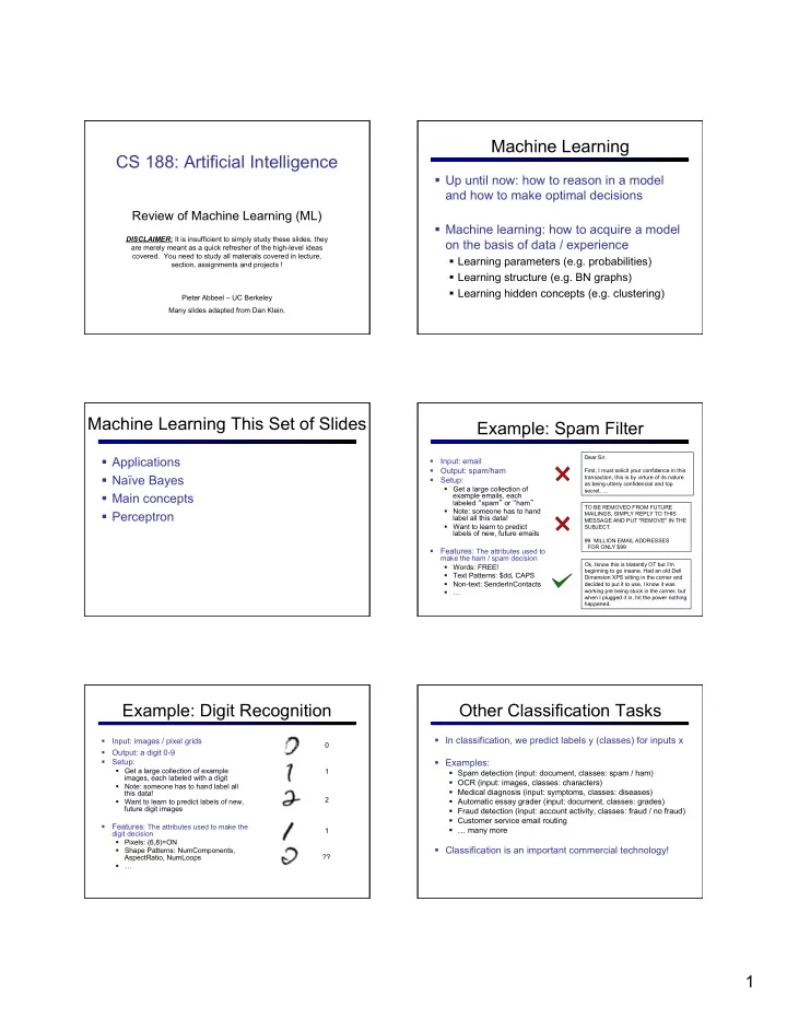
§ Input: email § Output: spam/ham § Setup:

§ Get a large collection of example emails, each labeled “spam” or “ham” § Note: someone has to hand label all this data! § Want to learn to predict labels of new, future emails

§ Features: The attributes used to

make the ham / spam decision § Words: FREE! § Text Patterns: $dd, CAPS § Non-text: SenderInContacts § …

Dear Sir. First, I must solicit your confidence in this transaction, this is by virture of its nature as being utterly confidencial and top

• secret. …

TO BE REMOVED FROM FUTURE MAILINGS, SIMPLY REPLY TO THIS MESSAGE AND PUT "REMOVE" IN THE SUBJECT. 99 MILLION EMAIL ADDRESSES FOR ONLY $99 Ok, Iknow this is blatantly OT but I'm beginning to go insane. Had an old Dell Dimension XPS sitting in the corner and decided to put it to use, I know it was working pre being stuck in the corner, but when I plugged it in, hit the power nothing happened.

Example: Digit Recognition

§ Input: images / pixel grids § Output: a digit 0-9 § Setup:

§ Get a large collection of example images, each labeled with a digit § Note: someone has to hand label all this data! § Want to learn to predict labels of new, future digit images

§ Features: The attributes used to make the

digit decision § Pixels: (6,8)=ON § Shape Patterns: NumComponents, AspectRatio, NumLoops § … 1 2 1 ??

Other Classification Tasks

§ In classification, we predict labels y (classes) for inputs x § Examples:

§ Spam detection (input: document, classes: spam / ham) § OCR (input: images, classes: characters) § Medical diagnosis (input: symptoms, classes: diseases) § Automatic essay grader (input: document, classes: grades) § Fraud detection (input: account activity, classes: fraud / no fraud) § Customer service email routing § … many more

§ Classification is an important commercial technology!

2

Bayes Nets for Classification

§ One method of classification:

§ Use a probabilistic model! § Features are observed random variables Fi § Y is the query variable § Use probabilistic inference to compute most likely Y

§ You already know how to do this inference

General Naïve Bayes

§ A general naive Bayes model: § We only specify how each feature depends on the class § Total number of parameters is linear in n

Y F1 Fn F2 |Y| parameters n x |F| x |Y| parameters |Y| x |F|n parameters

Inference for Naïve Bayes

§ Goal: compute posterior over causes

§ Step 1: get joint probability of causes and evidence § Step 2: get probability of evidence § Step 3: renormalize

+

A Digit Recognizer

§ Input: pixel grids § Output: a digit 0-9

Naïve Bayes for Digits

§ Simple version:

§ One feature Fij for each grid position <i,j> § Possible feature values are on / off, based on whether intensity is more or less than 0.5 in underlying image § Each input maps to a feature vector, e.g. § Here: lots of features, each is binary valued

§ Naïve Bayes model: § What do we need to learn?

Examples: CPTs

1 0.1 2 0.1 3 0.1 4 0.1 5 0.1 6 0.1 7 0.1 8 0.1 9 0.1 0.1 1 0.01 2 0.05 3 0.05 4 0.30 5 0.80 6 0.90 7 0.05 8 0.60 9 0.50 0.80 1 0.05 2 0.01 3 0.90 4 0.80 5 0.90 6 0.90 7 0.25 8 0.85 9 0.60 0.80

3

Naïve Bayes for Text

§ Bag-of-Words Naïve Bayes:

§ Predict unknown class label (spam vs. ham) § Assume evidence features (e.g. the words) are independent § Warning: subtly different assumptions than before!

§ Generative model § Tied distributions and bag-of-words

§ Usually, each variable gets its own conditional probability distribution P(F|Y) § In a bag-of-words model

§ Each position is identically distributed § All positions share the same conditional probs P(W|C) § Why make this assumption?

Word at position i, not ith word in the dictionary!

Example: Overfitting

2 wins!!

Example: Overfitting

§ Posteriors determined by relative probabilities (odds ratios):

south-west : inf nation : inf morally : inf nicely : inf extent : inf seriously : inf ...

What went wrong here?

screens : inf minute : inf guaranteed : inf $205.00 : inf delivery : inf signature : inf ...

Generalization and Overfitting

§ Relative frequency parameters will overfit the training data!

§ Just because we never saw a 3 with pixel (15,15) on during training doesn’t mean we won’t see it at test time § Unlikely that every occurrence of “minute” is 100% spam § Unlikely that every occurrence of “seriously” is 100% ham § What about all the words that don’t occur in the training set at all? § In general, we can’t go around giving unseen events zero probability

§ As an extreme case, imagine using the entire email as the only feature

§ Would get the training data perfect (if deterministic labeling) § Wouldn’t generalize at all § Just making the bag-of-words assumption gives us some generalization, but isn’t enough

§ To generalize better: we need to smooth or regularize the estimates

Estimation: Smoothing

§ Problems with maximum likelihood estimates:

§ If I flip a coin once, and it’s heads, what’s the estimate for P (heads)? § What if I flip 10 times with 8 heads? § What if I flip 10M times with 8M heads?

§ Basic idea:

§ We have some prior expectation about parameters (here, the probability of heads) § Given little evidence, we should skew towards our prior § Given a lot of evidence, we should listen to the data

Estimation: Smoothing

§ Relative frequencies are the maximum likelihood estimates § In Bayesian statistics, we think of the parameters as just another random variable, with its own distribution

????

4

Estimation: Laplace Smoothing

§ Laplace’s estimate:

§ Pretend you saw every outcome

• nce more than you actually did

§ Can derive this as a MAP estimate with Dirichlet priors (see cs281a)

H H T

Estimation: Laplace Smoothing

§ Laplace’s estimate (extended):

§ Pretend you saw every outcome k extra times § What’s Laplace with k = 0? § k is the strength of the prior

§ Laplace for conditionals:

§ Smooth each condition independently:

H H T

Estimation: Linear Interpolation

§ In practice, Laplace often performs poorly for P(X|Y):

§ When |X| is very large § When |Y| is very large

§ Another option: linear interpolation

§ Also get P(X) from the data § Make sure the estimate of P(X|Y) isn’t too different from P(X) § What if α is 0? 1?

Real NB: Smoothing

§ For real classification problems, smoothing is critical § New odds ratios:

helvetica : 11.4 seems : 10.8 group : 10.2 ago : 8.4 areas : 8.3 ... verdana : 28.8 Credit : 28.4 ORDER : 27.2 <FONT> : 26.9 money : 26.5 ...

Do these make more sense?

Tuning on Held-Out Data

§ Now we’ve got two kinds of unknowns

§ Parameters: the probabilities P(Y|X), P(Y) § Hyperparameters, like the amount of smoothing to do: k, α

§ Where to learn?

§ Learn parameters from training data § Must tune hyperparameters on different data

§ Why?

§ For each value of the hyperparameters, train and test on the held-out data § Choose the best value and do a final test

• n the test data

Important Concepts

§ Data: labeled instances, e.g. emails marked spam/ham

§ Training set § Held out set § Test set

§ Features: attribute-value pairs which characterize each x § Experimentation cycle

§ Learn parameters (e.g. model probabilities) on training set § (Tune hyperparameters on held-out set) § Compute accuracy of test set § Very important: never “peek” at the test set!

§ Evaluation

§ Accuracy: fraction of instances predicted correctly

§ Overfitting and generalization

§ Want a classifier which does well on test data § Overfitting: fitting the training data very closely, but not generalizing well

Training Data Held-Out Data Test Data

5

Generative vs. Discriminative

§ Generative classifiers:

§ E.g. naïve Bayes § A probabilistic model with evidence variables § Query model for class variable given evidence

§ Discriminative classifiers:

§ No generative model, no Bayes rule, often no probabilities at all! § Try to predict the label Y directly from X § Robust, accurate with varied features § Loosely: mistake driven rather than model driven

25

Binary Linear Decision Rule

§ Binary case: compare features to a weight vector § Learning: figure out the weight vector from examples

# free : 2 YOUR_NAME : 0 MISSPELLED : 2 FROM_FRIEND : 0 ... # free : 4 YOUR_NAME :-1 MISSPELLED : 1 FROM_FRIEND :-3 ... # free : 0 YOUR_NAME : 1 MISSPELLED : 1 FROM_FRIEND : 1 ...

Dot product positive means the positive class

Binary Linear Decision Rule

§ In the space of feature vectors

§ Examples are points § Any weight vector is a hyperplane § One side corresponds to Y=+1 § Other corresponds to Y=-1

BIAS : -3 free : 4 money : 2 ... 1 1 2 free money +1 = SPAM

• 1 = HAM

Binary Perceptron Update

§ Start with zero weights § For each training instance: § Classify with current weights § If correct (i.e., y=y*), no change! § If wrong: adjust the weight vector by adding or subtracting the feature vector. Subtract if y* is -1.

28

[demo]

Multiclass Linear Decision Rule

§ If we have multiple classes:

§ A weight vector for each class: § Score (activation) of a class y: § Prediction highest score wins

Binary = multiclass where the negative class has weight zero

Example Exercise --- Which Category is Chosen?

BIAS : -2 win : 4 game : 4 vote : 0 the : 0 ... BIAS : 1 win : 2 game : 0 vote : 4 the : 0 ... BIAS : 2 win : 0 game : 2 vote : 0 the : 0 ...

“win the vote”

BIAS : 1 win : 1 game : 0 vote : 1 the : 1 ...

6

Learning Multiclass Perceptron

§ Start with zero weights § Pick up training instances one by one § Classify with current weights § If correct, no change! § If wrong: lower score of wrong answer, raise score of right answer

31

Example

BIAS :1 win :0 game :0 vote :0 the :0 ... BIAS :0 win :0 game :0 vote :0 the :0 ... BIAS :-1 win :0 game :0 vote :0 the :0 ...

“win the vote” “win the election” “win the game”

Examples: Perceptron

§ Separable Case

33

Properties of Perceptrons

§ Separability: some parameters get the training set perfectly correct § Convergence: if the training is separable, perceptron will eventually converge (binary case) § Mistake Bound: the maximum number of mistakes (binary case) related to the margin or degree of separability Separable Non-Separable

34

Problems with the Perceptron

§ Noise: if the data isn’t separable, weights might thrash

§ Averaging weight vectors over time can help (averaged perceptron)

§ Mediocre generalization: finds a “barely” separating solution § Overtraining: test / held-out accuracy usually rises, then falls

§ Overtraining is a kind of overfitting

Fixing the Perceptron

§ Idea: adjust the weight update to mitigate these effects § MIRA*: choose an update size that fixes the current mistake… § … but, minimizes the change to w § The +1 helps to generalize

* Margin Infused Relaxed Algorithm

7

Minimum Correcting Update

min not τ=0, or would not have made an error, so min will be where equality holds

Maximum Step Size

38

§ In practice, it’s also bad to make updates that are too large § Example may be labeled incorrectly § You may not have enough features § Solution: cap the maximum possible value of τ with some constant C § Corresponds to an optimization that assumes non-separable data § Usually converges faster than perceptron § Usually better, especially on noisy data

Extension: Web Search

§ Information retrieval:

§ Given information needs, produce information § Includes, e.g. web search, question answering, and classic IR

§ Web search: not exactly classification, but rather ranking

x = “Apple Computers”

Feature-Based Ranking

x = “Apple Computers” x, x,

Now features depend on query and webpage. E.g.: #times word1 in query occurs, #times word2 in query occurs, #times all words in query

• ccur in sequence, …, page-rank

Perceptron for Ranking

§ Inputs § Candidates § Many feature vectors: § One weight vector:

§ Prediction: § Update (if wrong):

Classification: Comparison

§ Naïve Bayes

§ Builds a model training data § Gives prediction probabilities § Strong assumptions about feature independence § One pass through data (counting)

§ Perceptrons / MIRA:

§ Makes less assumptions about data § Mistake-driven learning § Multiple passes through data (prediction) § Often more accurate

42