M4500, February 10 Change of Bases Theorem Let J be the matrix of - - PowerPoint PPT Presentation

M4500, February 10

Change of Bases

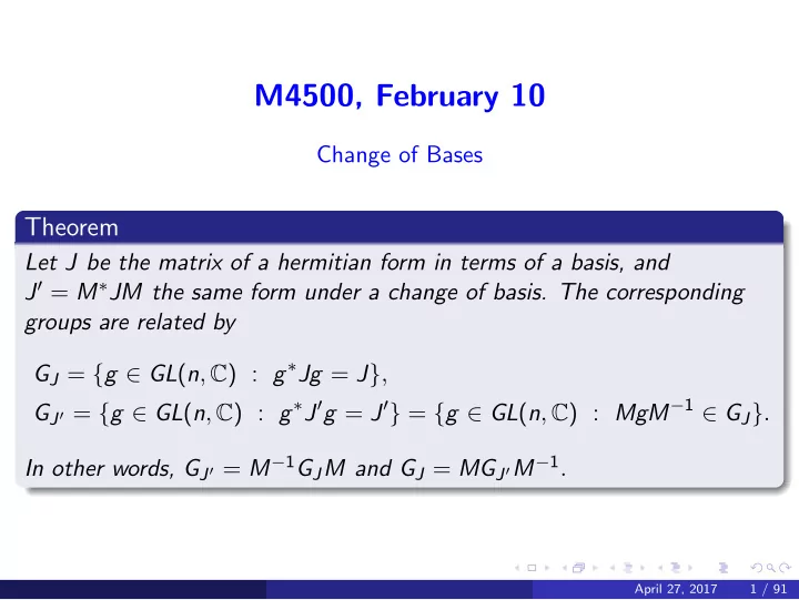
Theorem

Let J be the matrix of a hermitian form in terms of a basis, and J′ = M∗JM the same form under a change of basis. The corresponding groups are related by GJ = {g ∈ GL(n, C) : g∗Jg = J}, GJ′ = {g ∈ GL(n, C) : g∗J′g = J′} = {g ∈ GL(n, C) : MgM−1 ∈ GJ}. In other words, GJ′ = M−1GJM and GJ = MGJ′M−1.

April 27, 2017 1 / 91

O(1, 1) These are the 2 × 2 matrices of determinant 1 satisfying gTJ = Jg−1 : a c b d

• ·

1 −1

• =

1 −1

• ·

d −b −c a

• .

The resulting equations are a = d, b = c and a2 − b2 = 1. There are four types of matrices in O(1, 1), the first and last are in SO(1, 1). cosh t sinh t sinh t cosh t

• ,

− cosh t sinh t sinh t − cosh t

• ,

cosh t −sinht − sinh t cosh t

• ,
• So O(1, 1) has four connected components, SO(1, 1) has two. The same

happens for O(p, q), though somewhat harder to prove.

April 27, 2017 2 / 91

Coordinates for SL(2, R) The Euler Angles show that SO(3) is connected, and the analogues for SU(2) do the same. The HW problem indicates how this might generalize to SO(n) and SU(n). We do this for SL(2, R). Let e1 = 1

• . Then

StabSL(2,R)(e1) =

• n(x) :=

1 x 1

• .

Let g = a b c d

• ∈ SL(2, R). Then g ·

1

• =

a c

• = 0.

An arbitrary nonzero vector has polar coordinates a c

• =

r cos θ r sin θ

• ,. We

can write cos θ − sin θ sin θ cos θ

• ·

r r−1

• ·

1

• := r(θ) · a(r) ·

1

• =

a c

• = g ·

1

• .

April 27, 2017 3 / 91

So g−1 · r(θ) · a(r) ∈ StabSL(2,R)(e1), and any g is of the form g−1r(θ)a(r) = n(x) ⇐ ⇒ g = n(x)a(r−1)r(−θ). These are the coordinates we need to show SL(2, R) is connected.

April 27, 2017 4 / 91

O(n, 1) AT C T BT DT

• ·

I −I

• ·

A B C D

• =

I −I

• yields the equation BT · B − DT · D = −1. In turn this is

BTB = DTD − I ⇐ ⇒ b2

1 + · · · + b2 n = d2 − 1.

So either d ≥ 1 or d ≤ −1. If a path γ : [0, 1] ← → O(n, 1), γ(t) = A(t) B(t) C(t) D(t)

• goes from γ(0) = In+1×n+1 to some g, D(t) must stay ≥ 1. Any path that

contains a matrix with d ≤ −1, must stay that way. So there are at least 4 components, det = ±1 and d ≥ 1, d ≤ −1. Analogues of Euler Angles show that O(n, 1) has exactly 4 components.

April 27, 2017 5 / 91

Exercise 3.17 Compute   cos θ1 − sin θ1 sin θ1 cos θ1 1   ·   cosh t sinh t 1 cosh t sinh t   ·   cos θ2 − sin θ2 sin θ2 cos θ2 1   ·   1   .

April 27, 2017 6 / 91

Exercise 3.18 Compute r(θ1) · cosh t sinh t sinh t cosh t

• · r(θ2).

April 27, 2017 7 / 91

February 15 Connected component of the Identity Let G0 ⊂ G be the set of points that can be connected to I by a continuous path. Say γ(t), µ(t) ∈ G such that γ(0) = I, γ(1) = A and µ(0) = I, µ(1) = B. Then look at ρ(t) := [γ(t)]−1. It joins I with A−1. ρ(t) =

• µ(t)

0 ≤ t ≤ 1 A−1γ(t − 1)AB 1 ≤ t ≤ 2 joins I with AB; so does ρ(t) = γ(t) · µ(t). ρ(t) = gγ(t)g−1 joins I with gAg−1. You can use these path to show that G0 is a normal subgroup. The main point is that multiplication and inverses produce continuous paths out of continuous paths.

April 27, 2017 8 / 91

Exp and Log. To show that log ◦ exp and exp ◦ log are the identity, it is enough to do it for R. For exp ◦ log you need to substitute one series into the other; then collect powers of (x − 1) in

• 0≤n
• 1≤m(−1)m+1 (x−1)m

m

n n! . The coefficient of (x − 1)0 = 1 is 1. The coefficient of x − 1 is 1. The higher powers have coefficient 0. The answer is 1 + (x − 1) = x. It is VERY awkward to equate the coefficients. We can argue as follows: Within the radius of convergence, substituting and equating coefficients is justified to get the series for the composition of the functions. The Taylor series for exp and log are the listed ones. We know that exp and log are inverse to each other, therefore elog x = x = 1 + (x − 1) and log eX = X. These facts imply the answer for the coefficients. The calculation for x and X matrices is formally the same, so the answer follows.

April 27, 2017 9 / 91

February 17,2017 Quaternion Algebra

Definition

Q := {v = x0 + x1i + x2j + x3k}/{i2 = j2 = k2 = ijk = −1} Addition is done coordinate by coordinate, and multiplication is (x0 + x1i + x2j + x3k) · (y0 + y1i + y2j + y3k) = = (x0y0 − x1y1 − x2y2 − x3y3) + (x0y1 + x1y0 + x2y3 − x3y2)i+ + (x0y2 + x2y0 + x3y1 − x1y3)j + (x0y3 + x3y0 + x1y2 − x2y1)k, distributive and associative otherwise. The algebra has a conjugation, x0 + x1i + x2j + x3k = x0 − x1i − x2j − x3k and a norm |v|2 := v · v = x2

0 + x2 1 + x2 2 + x2 3.

April 27, 2017 10 / 91

Exercise. Show that every nonzero element has an inverse. Lie Algebra. The bracket (as for any associative algebra) is [v1, v2] := v1v2 − v2v1: 2(x2y3 − y2x3)i − 2(x1y3 − y1x3)j + 2(x1y2 − y1x2)k = det   i j k x1 x2 x3 y1 y2 y3   the cross product. So g := {x1i + x2j + x3k} forms a Lie subalgebra, in fact a Lie ideal. Exponential Map. Define exp(v) :=

• 0≤n

vn n! . You can ignore the x0; it commutes with everything, and just multiplies the exponential of the remainder by ex0. So we may as well restrict attention to g. Since v · v = v · v, 1 = exp(0) = exp(v + v) = exp(v) · exp(v). Since v = −v for v ∈ g, we can also conclude that exp(g) consists of elements of norm 1.

April 27, 2017 11 / 91

Exercise. What is the image of the exponential map? In the warmup you were asked to show that g ∼ = su(2) and that the elements of norm 1 are equivalent to SU(2).

April 27, 2017 12 / 91

February 22 A two dimensional Lie algebra has a basis {e1, e2}, and only one relation [e1, e2] = αe1 + βe2. If α = β = 0, this is the abelian Lie algebra. If not, may as well assume α = 0, by just interchanging the two basis vectors. Then e′

1 = e1 + β αe2

and e′

2 = 1 αe2 are also a basis. The bracket is

[e′

1, e′ 2] = 1

α[e1 + β αe2, e2] = 1 α (αe1 + βe2 + 0) = e1 + β αe2 = e′

1.

So there is only one up to equivalence, [e′

1, e′ 2] = e′ 1.

Check the 3−dimensional case, there are more cases, and su(2) as well as sl(2, R) have to show up.

April 27, 2017 13 / 91

• I + t

1!X + t2 2!X 2 + t3 3!X 3 + t4 4!X 4 + . . .

• ·

·

• I + t

1!Y + t2 2!Y 2 + t3 3!Y 3 + t4 4!Y 4 + . . .

• =

= I + t 1 1!X + 1 1!Y

• + +t2

1 2!X 2 1 1!1!XY + 1 2!Y 2

• +

+ t3 1 3!X 3 + 1 2!1!X 2Y + 1 1!2!XY 2 + 1 3!Y 3

• + . . .

April 27, 2017 14 / 91

For a Lie algebra g, you can define a liner map ad X : g − → g, ad X(Y ) = [X, Y ] It satisfies ad X ([Y , Z]) = [ad X(Y ), ad X(Z)] When g ⊂ M(n, F), is a Lie subalgebra, we have two linear maps, LX : M(n, F) − → M(n, F), LX(Y ) := XY , RX : M(n, F) − → M(n, F), RX(Y ) := YX. Tnen ad X = LX − RX. This has the advantage that LXRY = RY LX. Application: eX · Y · e−X = ead X(Y ).

April 27, 2017 15 / 91

Differential of Exp

For a map F = (f1, . . . , fm) : Rn − → Rm, the differential DF is the matrix DF := ∂fi ∂xj

• . We can compute it as a linear map at an x0 ∈ Rn :

DF(x0)(v0) = d dt

• t=0

F(x0 + tv0). We want to do this for F = exp : M(n, R) − → M(n, R). d dt

• t=0

eX+tY =

• n≥0

1 n!  

• 0≤k≤n−1

X kYX n−k−1   = =

• n≥0

1 n!  

• 0≤k≤n−1

Lk

XRn−k−1 X

  Y =

• n≥0

1 n! Ln

X − Rn X

LX − RX Y = = eLX − eRX ad X Y = eLX I − e− ad X ad X Y = eX I − e− ad X ad X Y .

April 27, 2017 16 / 91

Representations of Lie Algebras and Lie Groups

Any linear map into M(n, R) = gl(n, R) must be of the form φ(t) = tA. Two such representations are equivalent if the matrices differ by a change

• f basis; so this is the same as matrices up to similarity. The Lie group is

(R+, ×) with exponential map t → et. Any representation of the Lie algebra exponentiates Φ(et) = etA. On the other hand, we can consider G = (S1, ×). There is a dependence

• n the realization as a matrix group (which disappears if one considers it

as a Lie group). S1 := {r(θ) = cos θ − sin θ sin θ cos θ

• }

Lie(G) = { −θ θ

• }.

The Lie algebra is the same as before, realized differently. So the Lie homomorphisms are the same, φ : θ → θA. But for the group, Φ : θ → etA

• nly makes sense if e2πA = I.

April 27, 2017 17 / 91

General Definitions

Definition

A representation π : g − → gl(V ) or Π : G − → GL(V ) is called irreducible, if any subspace W ⊂ V which is left invariant by the action is either (0) or all of V . completely reducible, if any invariant subspace W ⊂ V has an invariant complement, V = W ⊕ W ′. It makes a difference if the vector space V is over R or C. A representation over a complex vector space V is called real if there is a real vector subspace VR ⊂ V satisfying dimR VR = dimC V which is invariant under the action. For the two examples and F = C, completely reducible means A is diagonalizable, and n = 1 is the only case when the representation can be irreducible.

April 27, 2017 18 / 91

Proposition

If a matrix satisfies e2πA = I, then A is diagonalizable. There are two proofs. The 2π is not relevant.

First Proof.

Find an invertible M so that MAM−1 is block upper triangular (Jordan canonical form/generalized eigenvectors). So A = S + N where S is diagonal,N upper triangular, and they commute. Then I = eA = eS+N = eSeN. This can only happen if N = 0. So A = M−1SM is diagonalizable.

April 27, 2017 19 / 91

Second Proof.

The group G = S1 is compact. Any compact group has a biinvariant measure dg, called Haar Measure. Let Π : G − → GL(V ). The claim is that V has a hermitian form , so that Π : G − → U(V , , ). Invariant Means

• G f (gx) dg =
• G f (xg) dg =
• G f (g) dg for any x ∈ G

and any continuoous function f : G − → C. Choose any inner product ( , ). Construct another one by the formula v1, v2

• G

(Π(g)v1, Π(g)v2) dg. The new one satisfies the requirements.

April 27, 2017 20 / 91

Adjoint Representation, Lie Algebra

Let g be a Lie subalgebra. The bracket is a bilinear map [ , ] : g × g − → g. So if we fix X ∈ g, and consider the bracket as a map in the second variable, we get a linear map denoted ad X : g − → g. Knowing the maps ad X is equivalent to knowing the bracket. The bracket satisfies the additional Jacobi identity. Check that this is equivalent to ad X([Y , Z]) = [ad X(Y ), Z] + [Y , ad X(Z)]. Write gl(g) for the linear transformations from g to g. This forms a Lie algebra in the usual way, [A, B] := AB − BA. The formula above is interpreted as saying that the map ad X : g − → g is a derivation. Given a Lie algebra g, we can define a subspace of gl(g) called Der(g) := {D ∈ gl(g) : D([X, Y ]) = [DX, Y ] + [X, DY ].

April 27, 2017 21 / 91

Derivations as Lie algebras

Check that the linear subspace of derivations is a Lie subalgebra of gl(g).

Proof.

We need to show that if D1, D2 ∈ Der(g), then [D1, D2] = D1 ◦ D2 − D2 ◦ D1 ∈ Der(g) : D1 ◦ D2([X1, X2]) = D1([D2X1, X2] + [X1, D2X2]) = = [D1D2X1, X2] + [D2X1, D1X2] + [D1X1, D2X2] + [X1, D1D2X2]. (D1D2 − D2D1)([X1, X2]) = [(D1D2 − D2D1)X1, X2] + [X1, (D1D2 − D2D1)X2].

Example

Differential operators of order less than or equal to 1 acting on functions: {D = a(x, y)+b(x, y)∂x +c(x, y)∂y}, DF(x, y) = aF +b∂xF +c∂yF. Question: What algebra is Span{1, mx, ∂x}?

April 27, 2017 22 / 91

Adjoint Representation, Lie Algebra

Exercise II. Viewing ad X as a function of X, we get a linear map ad : g − → gl(g). Check that the Jacobi identity translates into ad[X1, X2] = [ad X1, ad X2] := ad X1 ◦ ad X2 − ad X2 ◦ ad X1. This is interpreted as saying that ad : g − → Der(g) is a Lie homomorphism. Conclusion: Every Lie algebra structure defines a Lie homomorphism g − → Der(g) ⊂ gl(g) where the target has the usual bracket structure.

April 27, 2017 23 / 91

Adjoint Representation, Groups I

Exercise III. Let G ⊂ GL(n, R) be a matrix group with Lie algebra g ⊂ M(n, R); we also write M(n, R) = gl(n, R) to emphasize it is the Lie algebra of GL(n, R). For any element g ∈ G, we can define a continuous group homomorphism Ag : G − → G by the formula Ag(x) := gxg−1. Compute the differential dAg. This means you must calculate

d dt

• t=0 Ag(etX). Call the result Adg : g −

→ g. d dt

• t=0

getXg−1 = gXg−1. Left/Right multiplication Lg, Rg are linear maps on gl(n, R) their differentials are themselves. Verify directly using this formula that Ad g : g − → g is a Lie

• homomorphism. This means Ad g([X, Y ]) = [Ad g(X), Ad g(Y )]. Here

X, Y are n × n matrices and the bracket is the usual [A, B] = AB − BA.

April 27, 2017 24 / 91

Adjoint Representation, Groups II

You must also verify that if X ∈ g, then for any g ∈ G, gXg−1 ∈ g by using the definition of g : etgXg−1 = getXg−1. If g ∈ G and etX ∈ G, ∀t ∈ R, then the above formula shows gXg−1 ∈ g. Now consider the dependence in g ∈ G. Then Ad : G − → GL(g). Check that Ad(g1g2) = Ad g1 ◦ Ad g2 and Ad I = I. Be careful about the I

• n the left and the I on the right of the equation. In fact the image is in

Aut(g, [ , ]), invertible linear maps that commute with the bracket. The previous exercise shows that Ad : G − → GL(g) is a group

• homomorphism. It is fairly clear it is continuous.

Compute its differential. This means

d dt

• t=0 Ad(etX)(Y ). The answer is

ad X(Y ). We have in fact computed the differential of Ad and shown it is ad.

April 27, 2017 25 / 91

Ideals in Lie Algbebras I

Definition

A subalgebra h ⊂ g is called an ideal if [X, Y ] ∈ h for any X ∈ g, Y ∈ h.

Example

The center of the Lie algebra C(g) = z := {X ∈ g : [X, Y ] = 0 ∀ Y ∈ g} The derived algebra Dg = [g, g] := Span{X ∈ g : X = [Y , Z], for some X, Y ∈ g}. Central Series: C 0g := g, C n+1g := [g, C ng]. Nilpotent means C ng = 0 for large n. Derived Series: D0g := g, Dn+1g := [Dng, Dng]. Solvable means Dng = 0 for large n.

April 27, 2017 26 / 91

Ideals in Lie Algbebras II

Example

b = { upper triangular matrices } n = { strictly upper triangular matrices }

Theorem (Engel/Lie)

Any complex finite dimensional representation π : g − → gl(V ) of a solvable Lie algebra has a joint eigenvector. In other words there is a linear functional λ : g − → C and a 0 = v ∈ V such that π(X)v = λ(X)v. Any representation of a solvable Lie algebra has a basis such that all matrices are upper triangular.

Example (“Semisimple”, “Opposite” of Solvable)

g = sl(2, F) satisfies [g, g] = g.

April 27, 2017 27 / 91

Relation to Matrix Groups I

The analogue of ideal is normal subgroup. Let H ⊂ G be two matrix groups with Lie algebras h ⊂ g. Check that if H is normal, then h is an ideal.

Proof.

We need to show that if Y ∈ h and X ∈ g, then [X, Y ] ∈ h. This means etY ∈ H ⇒ et[X,Y ] ∈ H ∀t ∈ R. We know getY g−1 = etgYg−1. So if Y ∈ h, then gYg−1 ∈ h. This uses the definition of the Lie algebra. Set g = etX, and use the formula etXYe−tX = et ad XY ∈ h. Differentiate in t and set t = 0. This uses the definition of the derivative and the fact that h is a vector space.

April 27, 2017 28 / 91

Relation to Matrix Groups II

Check that if H ⊂ G are connected and h ⊂ g is an ideal, then H is a normal subgroup.

Proof.

As before, geY g−1 = egYg−1. If g = eX, then eXYe−X = ead X(Y ) ∈ h because ad X(Y ) = [X, Y ] ∈ h by virtue of h being an ideal. So for g = eX and h = eY , ghg−1 ∈ H. We know that exp is not always onto. However connected groups are generated by neighborhoods of the identity, and (g1g2)h(g1g2)−1 = g1(g2hg−1

2 )g−1 1 ,

g(h1h2)g−1 = gh1g−1gh2g−1. While expH, expG are not onto, any element is a product of terms of the form eX, eY . So the formulas above prove the claim.

April 27, 2017 29 / 91

Relation to Matrix Groups III

Remark

• 1. Recall the subgroup

eiθ eiαθ

• α /

∈ Q

• ⊂ S1 × S1.

This is NOT a matrix subgroup. However Π : S1 − → S1 × S1 given by the formula Π(eiθ) = eiθ eiαθ

• is a matrix group homomorphism, so the results about homomorphisms

still apply. 2. A discrete subgroup of a matrix group is a matrix group; its Lie algebra is (0), the machinery we developed is not useful.

April 27, 2017 30 / 91

Connectedness I

A set C ⊂ Rn is called connected if it cannot be decomposed as a disjoint union of two nonempty open sets C = U1 ∪ U2. Properties:

1 The notion is equivalent to Any open AND closed subset must be

either all of C or empty.

2 Pathwise Connected implies Connected. Any x1 ∈ U1 and x2 ∈ U2

must be connected by a continuous path γ : [0, 1] − → C, The inverse images γ−1(U1) and γ−1(U2) are nonempty, disjoint and open so unions of intervals. This is not possible.

3 If F : Rm −

→ Rn is continuous, then F(C) is connected as well.

April 27, 2017 31 / 91

Connectedness II

Theorem

Let G be a connected matrix group, and 0 ∈ U

exp

− − − − − − − →

∼ =

I ∈ V ⊂ G so that U is an open ball, and V = V−1. Then GV := {g1 · · · gn : gi ∈ V} = G. We say that G is is generated by V.

April 27, 2017 32 / 91

Connectedness III

Proof.

We show that GV is open and closed. It is open because for any element g = g1 · · · gn ∈ GV, gV ⊂ GV is an open neighborhood. It is closed because if xi − → g with xi ∈ GV, there has to be an xn ∈ gV. So xn = gx with xn, x ∈ V, and g = xnx−1 ∈ GV.

April 27, 2017 33 / 91

Representations of sl(2, C) I

Let (π, V ) be an irreducible representation of the Lie algebra sl(2, C). The relations [π(X), π(Y )] = π(X)π(Y ) − π(Y )π(X) are rewritten π(H)π(E) = 2π(E) + π(E)π(H), π(H)π(F) = −2π(F) + π(F)π(H), π(E)π(F) = π(H) + π(F)π(E). Because V is a complex finite dimensional vector space, π(H) must have an eigenvector. If π(H)vα = αvα, then π(H)π(E)vα = (2π(E) + π(E)π(H))vα = (2 + α)π(E)vα. So π(E)vα has eigenvalue α + 2. Similarly π(F)vα has eigenvalue α − 2. Since the dimension is finite and eigenvectors with distinct eigenvalues are

April 27, 2017 34 / 91

Representations of sl(2, C) II

independent, there must be a Λ such that π(H)vΛ = ΛvΛ, π(E)vΛ = 0. For more general situations of this type, Engel’s theorem is used. Let V ′ = Span {vΛ−2n := π(F)nvΛ} . We claim V ′ is invariant under π(sl(2, C)). Then V ′ = V . It is already clear that π(H) and π(F) leave V ′ invariant. So it is enough to show π(E)vΛ−2n is a multiple of vΛ−2n+2. The formal calculation is EF n = F nE + nF n−1(H − n + 1)). HF n = F n(H − 2n). So π(E)vΛ−2n = n(Λ − n + 1)vΛ−2n+2. Because dim V < ∞, there must be a smallest N such that π(F)vΛ−2N = 0. Then (Λ − 2N)vΛ−2N = π(H)vΛ−2N = π(E)π(F)vΛ−N − π(F)π(E)vΛ−2N = = −N(Λ − N + 1))vΛ−2N.

April 27, 2017 35 / 91

Representations of sl(2, C) III

This implies (N + 1)Λ = (N + 1)N, same as Λ = N is a nonnegative

• integer. The basis is vN, vN−2, . . . , v−N+2, v−N, and the dimension is

N + 1. From the warmup you computed the case N = 2.

Remark

For any Λ there is an infinite dimensional (highest weight module) module V (Λ) with basis vΛ−2n and formulas π(H)vΛ−2n = (Λ − 2n)vΛ−2n, π(F)vΛ−2n = vΛ−2n−2, π(E)vΛ−2n = n(Λ − n + 1)vΛ−2n+2. When Λ is an integer Λ = N, V (N) has a submodule V (−N − 2).

April 27, 2017 36 / 91

Representations of SL(2, C) I

There is a general representation of SL(2, F) on the space of functions f (x, y) by the formula (Π(g)f )(x, y) = f ((x, y) · g). We view (x, y) as a row vector. The meaning that this is a representation is: Π(g1g2)f (x, y) = f ((x, y)g1g2) = [Π(g2)f ]((x, y)g1) = = (Π(g1) [Π(g2)f ])(x, y)) . Let V (N) = Span

• fN−k(x, y) = xN−kyk

. This space has dimension N + 1, and the action of g = a b c d

• is

Π(g)xN−kyk = (ax + cy)N−k(bx + dy)k. The formula makes it clear that V (N) is invariant under the action of SL(2, C). Multiply out, all xαyβ have total degree α + β = N.

April 27, 2017 37 / 91

Representations of SL(2, C) II

Then Π 1 t 1

• xN−kyk = xN−k(tx + y)k

Π t t−1

• xN−kyk = tN−2kxN−kyk

Π 1 t 1

• xN−kyk = (x + ty)N−kyk

The differential π := dΠ is π 1

• xN−kyk = kxN−k+1yk−1

π 1 −1

• xN−kyk = (N − 2k)xN−kyk

π 1

• xN−kyk = N − kxN−k−1yk+1

April 27, 2017 38 / 91

Representations of SL(2, C) III

This is just the rescaled version of the vN−2k from before: vN−2k = 1 (N − k)!fN−k.

Exercise

Write down the formulas for π(H), π(E) and π(F) in the two bases.

April 27, 2017 39 / 91

Representations of SU(2)

It is clear that SU(2) ⊂ SL(2, C), so the representations restrict to this group.

Theorem

The representations V (N) of SU(2) and SL(2, C) are irreducible.

Proof.

If there were an invariant V ′ ⊂ V , it would also be invariant under the Lie

• algebra. But the representation of the Lie algebra is irreducible. The

crucial fact about the Lie algebra is su(2) + isu(2) = sl(2, C).

April 27, 2017 40 / 91

Representations of SO(3)

Recall that 1 − → {±I} − → SU(2)

p

− → SO(3) − → 1. If the matrices Π(±I) = I(N+1)×(N+1), then V (N) drops down to a representation of SO(3).

Lemma

A representation of a connected matrix group is is irreducible if and only if the corresponding representation of the Lie algebra is irreducible.

Proof.

This uses the fact that a connected group is generated by a neighborhood

• f the identity.

Corollary

Π(±I) = I(N+1)×(N+1) if and only if N is even.

Proof.

The key fact is that dp is an isomorphism of Lie algebras.

April 27, 2017 41 / 91

Schur’s Lemma

Theorem

Assume (π, V ) is an irreducible representation on a complex vector space. If A : V − → V satisfies A ◦ π(X) = π(X) ◦ A for all X ∈ g (or for a group representation), then A is a multiple of the identity.

Proof.

Let Vλ := {v ∈ V : Av = λv}, the λ−eigenspace of A. There is λ ∈ C such that Vλ = (0). This space is invariant under the action of g : Aπ(X)v = π(X)Av = λπ(X)v. Since it is = (0) Vλ = V .

April 27, 2017 42 / 91

Casimir Operator

Consider the formal expression Ω := H2 + 2(EF + FE). While it may not make sense formally, it gives rise to an operator π(Ω) on any representation (π, V ): π(Ω) = π(H)2 + 2(π(E)π(F) + π(F)π(E)).

Proposition

π(Ω)π(X) = π(X)π(Ω) for any X ∈ g.

Proof.

π(X)π(Ω) − π(Ω)π(X) = [π(X), π(Ω)] = ad π(X)(π(Ω)). For matrices ad X(Y1 · · · Yn) = XY1 · · · Yn − Y1 · · · YnX = =

• Y1 · · · Yk−1XYkYk+1 · · · Yn − Y1 · · · Yk−1YkXYk+1 · · · Yn =

=

• Y1 · · · Yk−1 ad X(Yk)Yk+1 · · · Yn.

Apply this to X = E, H, F, and Ω get 0 each time.

April 27, 2017 43 / 91

Complete Reducibility I

For πN, V (N), the value can be computed on vN : π(Ω)vN = [(N + 1)2 − 1]vN. Any representation will decompose into a direct sum of (generalized) eigenspaces for π(Ω). Any generalized eigenspace must have eigenvalue [(N + 1)2 − 1]; call it V N. Any invariant irreducible subspace of V N must be a V (N). Two such subspaces must either coincide or have intersection

• 0. This almost implies that V N is direct sum of V (N)’s. The next

theorem is what is missing.

Theorem

Suppose 0 − → V1 − → V − → V2 − → 0 is an exact sequence of modules such that V1, V2 ∼ = V (N). Then V is a direct sum of V1 and V2.

April 27, 2017 44 / 91

Complete Reducibility II

Proof.

The generalized eigenvalues of H are N, N − 2, . . . , −N + 2, −N, and E raises the generalized eigenvalue by 2, F lowers it by 2. The problem is that the N−eigenspace of H may not be semisimple. If it is, the previous arguments prove the theorem. So assume there is v′ such that v = (H − N)v′ = 0 and Hv = Nv. The space {F nv} is an invariant irreducible subspace by the previous calculations. In particular Ev = 0, F Nv = 0, F N+1v = 0. Then: ad E(F n) =

n−1

• k=0

F kHF n−k−1 =

• F n−1(H − 2n + 2k + 2) =

= nF n−1(H − n + 1), 0 = EF N+1v′ = F N+1Ev′ + (N + 1)F N(H − N)v′ = 0 + (N + 1)F Nv. It follows that F Nv = 0, a contradiction.

April 27, 2017 45 / 91

The Enveloping Algebra

This is an aside, not many proofs. This notion justifies why we can dispense with π(X) and multiply elements of the Lie algebra. We embed g in an associative Lie algebra U(g) with unit so that the Lie algebra structures are compatible. First recall T(g) =

• g ⊗ · · · ⊗ g
• n

. For n = 0, the factor is C. This is an associative algebra under concatenation of

• tensors. There is an obvious map ǫ : g −

→ T(g). Any linear map f : g − → A (an associative algebra with unit) extends uniquely to an algebra map T(g) − → A satisfying 1 → 1 and X → f (X). Define U(g) := T(g)/ {T(g)[X ⊗ Y − Y ⊗ X − [X, Y ]]T(g)}. Then ǫ induces a Lie algebra map g − → U(g) which is an inclusion.

Theorem

Any representation of g extends uniquely to a representation of U(g) as an algebra, 1 → I, X → π(X), XY → π(X)π(Y ). In U(g), [ǫ(X), ǫ(Y )] = ǫ(X)ǫ(Y ) − ǫ(Y )ǫ(X).

April 27, 2017 46 / 91

Matrix Entries

Let H ⊂ G be two groups. Let F(G) or F(G/H) be a space of functions

• n G, or on G/H, for example continuous, or integrable or L2 (assuming

an invariant measure). There is a natural representation Lg(f )(x) := f (g−1x). This time it has to be g−1 to satisfy Lg1g2 = Lg1 ◦ Lg2. Assume (π, V ) is a unitary representation of G, with basis {e1, . . . , eN}, possibly orthonormal. We define matrix entries fei,ej = fij(g) := π(g)ej, ei. More general for v, w ∈ V , define fv,w := π(g)w, v. Suppose there is a vector v0 ∈ V such that π(h)v0 = v0, ∀h ∈ H. Then fv,v0 ∈ F(G/H).

Example

In the case of G = S1, the irreducible representations are πn(eiθ) = einθ. So the matrix entries are fn(eiθ) = einθ

• themselves. Fourier Series is about representing functions on the circle as

April 27, 2017 47 / 91

Some Remarks I

For G = S1, F(G) are L2−functions. An irreducible representation has to be 1-dimensional because any finite dimensional representation is completely reducible (look up the slide about integration). Fourier series is f (eiθ) → aneinθ, and an =

1 2π

2π f (eiθ)e−iθ dθ. The issue is how the series approximates the function. We do not need the representation to be unitary. If (π, V ) is a representation of a group, let V ∗ := {λ : V − → C : λ linear}. Then we can define a representation (π∗, V ∗) by the formula (π∗(g)λ)(X) = λ(π(g−1)X). Similarly for a Lie algebra (π(X)λ)(Y ) = λ(−π(X)Y ). Note that the second one is the differential of the first one. Matrix Entries would be fλ,v(g) = (λ(π(g−1)v). F(G) inherits a representation of G × G : (Rg1,g2f )(x) = f (g−1

1 xg2).

April 27, 2017 48 / 91

Some Remarks II

In general, say π(g)ej = fij(g)ei, and {ek} is orthonormal. Then fij(g) = π(g)ej, ei. Furthermore, fei,ej(g1g2) = π(g1)π(g2)ej, ei =

• fkj(g2)π(g1)ek, ei =

=

• fmk(g1)fkj(g2)em, ei =
• fik(g1)fkj(g2).

The way to remember this is π(g1) ◦ π(g2) = π(g1g2) written as matrices. For a unitary representation, fij(g) = fji(g−1) as well. One of the motivations for writing these formulas, is that in coordinates matrix entries are special functions occuring in Mathematical Physics and Applied Mathematics. They satisfy relations which are hard to derive computationally, but are clear from this point of view. We see this in the next examples.

April 27, 2017 49 / 91

The Examples of SU(2), SO(3), S2 I

Let P be the vector space of polynomials in two variables. There is an action of SL(2, C) by the formula g · f (x, y) = f ((x, y) · g), and P = V (N). P also comes with a symmetric bilinear form, (p, q) := ∂p(q)(0). This form is nondegenerate, with an orthonormal basis xαyβ √α!β!. This IS NOT an inner product. The following relations are clear: (xp, q) = (p, ∂xq), (yp, q) = (p, ∂yq). The action of the Lie algebra sl(2, C) is E ← → x∂y, H ← → x∂x − y∂y, F ← → y∂x. So since (x∂xp, q) = (p, x∂xq), (H · p, q) = +(p, H · q), (E · p, q) = (p, F · q).

April 27, 2017 50 / 91

The Examples of SU(2), SO(3), S2 II

There is an inner product, p, q := (p, q).

Exercise

Show that π(g) for g ∈ SU(2) are unitary for , .

Proof.

iH · p, q = −p, iH · q, (E − F) · p, q = −p, (E − F) · q, i(E + F) · p, q = −p, i(E + F) · q. Recall g = r(φ) · t(θ) · r(ψ), with 0 ≤ φ < 2π, 0 ≤ φ < π, 0 ≤ ψ < 2π : g = eiφ/2 e−iφ/2

• ·

cos θ

2

i sin θ

2

i sin θ

2

cos θ

2

• ·

.eiψ/2 e−iψ/2

• April 27, 2017

51 / 91

The Examples of SU(2), SO(3), S2 III

In the literature, N = 2ℓ, and the H, E, F are rescaled, and often a different basis adapted to su(2) or so(3) is used. Also Ω is replaced by Ω

4 .

The formulas are π(H/2)xℓ−kyℓ+k = (ℓ − k)xℓ−kyℓ+k π(E)xℓ−kyℓ+k = −(ℓ − k)xℓ−k+1yℓ+k−1 π(F)xℓ−kyℓ+k = −(ℓ + k)xℓ−k−1yℓ+k+1 π(Ω)xℓ−kyℓ+k = ℓ(ℓ + 1)xℓ−kyℓ+k xℓ−kyℓ+k, xℓ−kyℓ+k = (ℓ + k)!(ℓ − k)!.

April 27, 2017 52 / 91

Matrix Entries I

The functions fp,q(g) = π(g)q, p are the matrix entries defined earlier. Specialize to the basis ek =

xN−kyk

√

k!(N−k)! to get functions Ym,n on

SU(2) = S3. In particular for N even, these are functions on SO(3). Using N even and n = 0 gives functions fn,0 on S2. Switch to N = 2ℓ with ℓ ∈ N, and xℓ−nyℓ+n.

Exercise

Write the functions fn,0 in spherical coordinates. These turn out to be examples of Legendre polynomials. Use the coordinates in SU(2) and SO(3) that we studied earlier. Later we bring in spherical coordinates to interpret the matrix entries as functions

• n the sphere. The function fn0 satisfies

fm0(g) = π(r(φ) · t(θ) · r(ψ)e0, em = π(r(t(θ)))e0, π(r(−φ))em = = ei(ℓ−m)φfm0(t(θ)).

April 27, 2017 53 / 91

Matrix Entries II

So it is determined by its values on t(θ). Up to xℓ−myℓ+m, xℓ−myℓ+m, fm0(t(θ)) = π(t(θ)e0, em = = (cos θ 2x + i sin θ 2y)ℓ(i sin θ 2x + cos θ 2)ℓ, xℓ−myℓ+m =

• 0≤b≤ℓ−m

ℓ b

• ℓ

ℓ − m − b

• (i)m+2b
• cos θ

2 2ℓ−m−2b sin θ 2 m+2b . When you substitute cos2 θ 2 = 1 + z 2 , sin2 θ 2 = 1 − z 2 , The resulting function in z is a Legendre Polynomial. The relations between Legendre polynomials are just the formulas on page 51. The special case m = 0 is called a zonal spherical function.

April 27, 2017 54 / 91

Spherical Coordinates

The infinitesimal operators can be rewritten as differntial operators. The matrix entries for representations of SO(3) are determind by their values

• n the sphere x2 + y2 + z2 = 1. They come from representations V (N)

with N even, and are of the form fn,0 = π(g)e0, en. Since SO(3)/SO(2) ∼ = S2, we can write them in spherical coordinates. Coordinates: x = r sin φ cos θ y = r sin φ sin θ z = r cos φ Jacobian:   ∂r/∂x = sin φ cos θ ∂φ/∂x = cos φ cos θ/r ∂θ/∂x = − sin θ/(r sin φ) ∂r/∂y = sin φ sin θ ∂φ/∂y = cos φ sin θ/r ∂θ/∂y = cos θ/(r sin φ) ∂r/∂z = cos φ ∂φ/∂z = − sin φ/r ∂θ/∂z = 0  

April 27, 2017 55 / 91

Action of the Algebra I

su(2) a1 = 1 2 i i

• a2 = 1

2 1 −1

• a3 = 1

2 i −i

• so(3)

A1 =   1 −1   A2 =   −1 1   A3 =   1 −1   Action on functions f : R3 − → C : (X · F)(x) := d dt

• t=0

f (e−tXx). A1 − → y∂z − z∂y, A2 − → z∂x − x∂z, A3 − → x∂y − y∂x Note that A1 + iA2 ← → iE, A1 − iA2 ← → iF, −2iA3 ← → H.

April 27, 2017 56 / 91

Action of the Algebra II

In spherical coordinates (NOTE the absence of ∂r, and 0 ≤ φ < 2π and 0 ≤ θ < π are interchanged from the usual spherical coordinates) A1 − → − sin φ∂θ − cot θ∂φ, A2 − → cos φ∂θ − cotθ sin φ∂φ, A3 − → ∂φ. In these coordinates, −Ω/4 = a2

1 + a2 2 + a2 3 :

1 sin θ ∂ ∂θ

• sin θ ∂

∂θ

• +

1 sin2 θ ∂2 ∂2φ. Make the change of variables t = cos θ, with 0 ≤ θ ≤ π, and plug in a function eimφΘ(θ) : (1 − t2)d2Θ dt2 − 2t dΘ dt +

• ℓ(ℓ + 1) −

m2 1 − t2

• Θ = 0.

is called the Legendre Equation.

April 27, 2017 57 / 91

Spherical Harmonics I

Compare this with the formula of the Laplacian ∇2 = ∂2

x + ∂2 y + ∂2 z in

spherical coordinates: ∇2 = 1 r2 ∂ ∂r

• r2 ∂

∂r

• +

1 r2 sin θ ∂ ∂θ

• sin θ ∂

∂θ

• +

1 r2 sin2 θ ∂2 ∂2φ. We want to solve ∇2F(x, y, z) = 0, and F should be regular throughout

• R3. We can use spherical coordinates. The standard way is to use

separation of variables F = f (r)Y (θ, φ). The solution space is a representation of SO(3) which only acts on Y . This makes the separation

• f variables more natural.

1 f ∂ ∂r

• r2 ∂f

∂r

• = λ,

1 Y ∇SY = −λ.

April 27, 2017 58 / 91

Spherical Harmonics II

We can separate further Y = Φ(φ)Θ(θ) : 1 Φ d2Φ dφ2 = −m2 λ sin2 θ + 1 Θ d dθ

• sin θdΘ

dθ

• = m2.

m is complex, but Φ must be periodic with period 2π, so we can take it to be a nonnegative integer, and therefore Φ(φ) is a linear combination of e±imφ.

April 27, 2017 59 / 91

Harmonic Polynomials I

∇2f = 0 where ∇2 = ∂2

x + ∂2 y + ∂2 z , is called the Laplace Equation. We

want to compute the solutions which are polynomial. The vector space is denoted H. It is a representation of SO(3) because ∇2Lgf = Lg∇2f , and decomposes, according to homogeneous degree, as H = H(N). The polynomial r2 = x2 + y2 + z2 is invariant under the action of SO(3), and there is an orthogonal decomposition P(N) = H′(N) + r2P(N − 2).

Lemma

H′(N) = H(N).

Proof.

The inner product is p, q = ∂p(q)(0). The relation ∇2p, q = p, r2q holds. The dimension is dim H(N) = (N+1)(N+2)

2

− (N−1)N

2

= 2N + 1. We can find a harmonic polynomial hN := (x + iy)N, and check that A3 · hN = iNhN

April 27, 2017 60 / 91

Harmonic Polynomials II

and E · hN = (A2 − iA3)hN = 0. This vector generates an irreducible module for SO(3, C) ∼ = sl(2, C) of dimension 2N + 1. So H(N) ∼ = V (2N). One can compute a basis for the module by applying F = A2 + iA3

• repeatedly. These are the function fn0 from before, up to rescaling.
• QUESTION. Why are these functions the fn0 from before.

April 27, 2017 61 / 91

Types of Representations I

G a matrix group, (π, V ) a unitary representation, {e1, . . . , eN} an

• rthonormal basis.

π(g)ej =

• fkj(g)ek,

fij(g1g2) =

• k

fik(g1)fkj(g2), (Lgfij)(x) = fij(g−1x) =

• k

fik(g−1)fkj(x), Rgfij(x) = fij(xg) =

• k

fik(x)fkj(g) =

• k

fkj(g)fik(x). Fix i in the fourth formula. The conclusion is that Span{fij} is invariant under the right action. The map ej → fij is well defined because the ej form a basis, and gives an intertwining operator. If (π, V ) is irreducible, then the fij are linearly independent.

April 27, 2017 62 / 91

Types of Representations II

Fix j in the third formula. Then Span{fkj} is invariant under Lg. This is also a representation, but which one? Dual Let V ∗ := {λ : V − → C : λ complex linear}. If V is a representation, define π∗(λ)(v) := λ(π(g−1)v). Hermitian Dual Let V h := {λ : V − → C : λ conjugate linear }, i.e. λ(αv1 + βv2) = αλ(v1) + βλ(v2). This is a complex vector space, (c · λ)(v) := cλ(v), and a representation by the same formula as for the dual. If V admits a hermitian form, then V ∼ = V h, NOT V ∗. Tensor Product If (V1, π1) and (V2, π2) are representations of G1, G2, (π1 ⊗ π2)(g1, g2)v1 ⊗ v2 := π1(g1)v2 ⊗ π2(g2)v2. Hom Let HomC[V1, V2] be the vector space of C−linear maps from V1 to V2. This carries a representation of G1 × G2: Hπ1,π2(g1, g2)A = π2(g2) ◦ A ◦ π1(g−1

1 ).

April 27, 2017 63 / 91

Types of Representations III

Choose a basis {e1, . . . , eN} of the representation (π, V ). Then V ∗ has a dual basis {λ1, . . . , λN} satisfying λi(ej) := δij. Matrix entries are written as fij(g) = λi(π(g−1)ej). The formulas are π(g)ej =

• fkj(g)ek,

fij(g1g2) =

• k

fik(g1)fkj(g2), π∗(g)λi =

• k

fik(g−1)λk (Lgfij)(x) = fij(g−1x) =

• k

fik(g−1)fkj(x),

April 27, 2017 64 / 91

Types of Representations IV

The formula in red comes from the following calculation: [π∗(g)λi] =

• cikλk ⇐

⇒ cik = [π∗(g)λi](ek) [π∗(g)λi](ek) = λi(π(g−1)ek) = λi(

• ℓ

fℓk(g−1eℓ) = fik(g−1), π∗(g)λi =

• k

fik(g−1)λk. If you fix j, then (Lg, Span{fkj})) matches V ∗.

April 27, 2017 65 / 91

Types of Representations V

Example

For SU(2) there is only one irreducible representation for each dimension. If (π, V ) is irreducible, so are π∗ and πh. Let G = SU(3), and define (π, V ) to be V ∼ = C3 as column vectors, π(g)v = g · v. The dual vector space is V ∗ ∼ = C3 but this time realized as row vectors. So (λ1, λ2, λ3) represents a linear function, λ(v) = λ · v. The representation π∗ is π∗(λ) := λ · g−1. Then π and π∗ are not equivalent (isomorphic). This follows from the lemma below.

Lemma

Let (π1, V1) and (π2, V2) be isomorphic representations. Then Tr π1(g) = Tr π2(g) ∀g ∈ G.

April 27, 2017 66 / 91

Types of Representations VI

Proof.

By assumption there is A : V1

∼ =

− → V2. Identify V1 = V2 = V . Then A ◦ π1(g) = π2(g) ◦ A ⇐ ⇒ π2(g) = A ◦ π1(g) ◦ A−1. Then Tr π2(g) = Tr(A ◦ π1(g) ◦ A−1 = Tr π1(g). For an element of the form g = diag(eiφ, eiθ, eiψ), we compute Tr π(g) = eiφ + eiθ + eiψ, and Tr π∗(g) = e−iφ + e−iθ + e−iψ.

April 27, 2017 67 / 91

Tensor Products and Matrix Entries I

If we consider the full Span{fij}, then G × G acts by Lg ⊗ Rg, and we get a representation isomorphic to V ∗ ⊗ V . For finite dimensional spaces, there is an isomorphism V ∗

1 ⊗ V2 ∼

= HomC[V1, V2], λ ⊗ v2 → Fλ⊗v2(v1) := λ(v1)v2.

Theorem

If (π1, V1) and (π2, V2) are irreducible representations of G1 and G2 respectively, then (π1 ⊗ π2, V1 ⊗ V2) is an irreducible representation of G1 × G2. Conversely, any irreducible representation of G1 × G2 is of this form. This is one of the basic facts of representation theory. The proof can be found in abstract (noncommutative) algebra books, known as the Jacobson density theorem.

April 27, 2017 68 / 91

Tensor Products and Matrix Entries II

As already mentioned, you can think of matrix entries as functions attached to elements λ ⊗ v ∈ V ∗ ⊗ V : fλ,v(g) := λ(π(g−1)v). In other words there is an operator Aπ : V ∗ ⊗ V − → F(G), λ ⊗ v → fλ⊗v(g) := λ(π(g)−1v) which intertwines π∗ ⊗ π with (Lg, Rg). It is better to use HomC[V , V ]. For A ∈ HomC[V , V ], define the function fA(g) := Tr(π(g) ◦ A). Problem: Let G1 = G2 = G, and (π1, V1) and (π2, V2) be irreducible

• representations. Then G embeds in G × G as the diagonal.

Decompose V1 ⊗ V2 into irreducible representations of G. Clebsch-Gordan coefficients are an instance of this problem. The group is G = SU(2), and you want to decompose the tensor product of any two of its representations.

April 27, 2017 69 / 91

Tensor Products and Matrix Entries III

The more general version, a basic problem in representation theory, is: Let H ⊂ G be a subgroup and (π, V ) a representation. Decompose V into irreducible representations of H.

April 27, 2017 70 / 91

Schur Orthogonality Relations I

Lemma (Schur’s Lemma)

Let (π1, V1) and (π2, V2) be irreducible representations. Any intertwining

• perator A : V1 −

→ V2 i.e. linear which satisfies A ◦ π1(g) = π2(g) ◦ A is a “multiple of the identity”. So either there is no such operator other than A = 0, in which case we say the representation are inequivalent, or there is a nonzero one, in which case we can identify V1 = V2 = V , and π1 = π2; then A = λI for some λ ∈ C.

April 27, 2017 71 / 91

Schur Orthogonality Relations II

Theorem (Schur Orthogonality Relations)

Let (π1, V1) and (π2, V2) be irreducible representations, and fij, hkl be matrix entries with respect to orthonormal bases. If π1 and π2 are inequivalent,

• G

fij(g)hkl(g) dg = 0 ∀i, j, k, l. Assume π1 = π2 = π and V1 = V2 = V . Then

• G

fij(g)fkl(g) dg = δik · δjl dim V . We assume that

• G dg = 1.

April 27, 2017 72 / 91

Schur Orthogonality Relations III

Proof.

Let A : V1 − → V2 be any linear map. We can associate an intertwining

• perator

A :=

• G

π2(g) ◦ A ◦ π1(g−1) dg. If V1 ∼ = V2, A = 0. If V1 = V2 = V , apply the trace. On the one hand A = λI, so Tr A = λ dim V , On the other hand, Tr

• G

π(g) ◦ A ◦ π(g−1) dg

• =
• G

Tr

• π(g) ◦ A ◦ π(g−1)
• dg =

=

• G

Tr

• A ◦ π(g−1) ◦ π(g)
• dg = Tr A.

So Tr A = λ dim V = Tr A. Thus λ =

Tr A dim V .

The relations follow from choosing all possible A.

April 27, 2017 73 / 91

Schur Orthogonality Relations IV

Example

Suppose dim V1 = 2 and dim V2 = 3. Choosing bases, π1(g) = f11(g) f12(g) f21(g) f22(g)

• ,

π2(g) =   h11(g) h12(g) h13(g) h21(g) h22(g) h23(g) h31(g) h32(g) h33(g)   , A = E12 :=   1   . Then π2(g) ◦ E12 ◦ π1(g)−1 =   h11(g)f21(g−1) h11(g)f22(g−1) h21(g)f21(g−1) h21(g)f22(g−1) h31(g)f21(g−1) h31(g)f22(g−1)  . Use fij(g−1) = fji(g) and integrate each entry separately. Since a 3−dimensional and a 2−dimensional vector space cannot be isomorphic, all the integrals are 0.

April 27, 2017 74 / 91

Characters

For each representation π, V ), define the Character of π to be χπ(g) = Tr π(g). This is a class function meaning it satisfies f (gxg−1) = f (x) for all x, g ∈ G. For irreducible modules

• G

χπ1(g)χπ2(g) dg =

• 1

if π1 ∼ = π2, if π1 ∼ = π2. This follows from writing χπ(g) = fii(g) in terms of the matrix entries, and using the Schur orthogonality relations.

Exercise

Compute χπ(N) for G = SU(2). In principle, knowledge of the characters of the irreducible representations

• f a compact group, solves the main problems of representation theory.

April 27, 2017 75 / 91

The Peter-Weyl Theorem I

This is a basic result of the Representation Theory of compact groups. In particular it applies to finite groups. The main reference is the text by Br¨

• cker-tomDieck, there are many more.

Theorem

Let M := Span{f π

ij

: fij matrix entries of π irreducible }. Then M ⊂ L2(G) is dense. For a function f ∈ L2(G), define the matrix coefficients to be cπ

ij (f ) :=

• G f (g)f π

ij (g) dg. Then

f (g) =

• π,i,j

cπ

ij (f )f π ij (g).

If f is continuous, then convergence is uniform.

April 27, 2017 76 / 91

The Peter-Weyl Theorem II

Proof.

Suppose Cl(M) = L2(G). Then there is an orthogonal complement 0 = H ⊂ L2(G). We show that this leads to a contradiction. First, H is invariant under the right regular action Rg. The basic fact is that any invariant space contains a nontrivial irreducible finite dimensional representation (π, V ). In our case, H is realized as functions on G. Choose an orthonormal basis {e1, . . . , eN} of V . Then Rg(ej)(x) = ej(xg) =

• f π

ij (g)ei(x),

∀x, g ∈ G Set x = 1 : ej(g) =

• ei(1)f π

ij (g).

This says that all of the ej are linear combinations of the f π

ij . So they (and

all of V ) are in M ∩ H = (0).

April 27, 2017 77 / 91

The Peter-Weyl Theorem III

The fact that any invariant subspace must contain a nontrivial finite dimensional invariant subspace is trivial when G is finite; L2(G) = F(G) is itself finite dimensional. In general you need the theory of compact self adjoint operators on Hilbert spaces. See the lecture notes of the course for a summary, and Br¨ cker-tomDieck for carefully spelled out details.

April 27, 2017 78 / 91

Consequences I

Let (π, V ) be a finite dimensional representation of a compact group. It is completely reducible, V = ⊕Vj where each (πj, Vj) is irreducible. We want to know how many copies of a particular (ρ, W ) occur in the

• decomposition. The character of (π, V ) equals χV = mjVj. Then

χρ, χπ = mρ.

Example

G = SU(2), to (πm, V (m)) and (πn, V (n)) we can associate (πm ⊗ πn, V (m) ⊗ V (n)). Its character is χm · χn. We can compute,  

• −m≤s≤m

ei(m−s)θ   ·  

−n≤t≤n

ei(n−t)θ   =

m+n

• ℓ=|m−n|

χℓ. In the sum the ℓ go down by 1.

April 27, 2017 79 / 91

Consequences II

In Physics, the explicit decomposition of the tensor product in terms of bases of V (m) and V (n) are important. Look up Clebsch-Gordan coefficients for details. A basic case is V (n = 1/2) the 2−dimensional irreducible representation: V (m) ⊗ V (1/2) = V (m + 1/2) + V (m − 1/2). Also V (m) ⊗ V (1) = V (m + 1) + V (m) + V (m − 1).

April 27, 2017 80 / 91

Finite Groups I

The case of finite groups is very important. The Peter Weyl theorem is

• easier. But the information about specific groups is quite difficult.

Example

Let G = S4 and H = S3 ⊂ G. You can restrict a representation (π, V ) of G to H; what is its composition series in terms of irreducible representations of H? Haar Measure:

• G

f (x) dx = 1 |G|

• x∈G

f (x). For x ∈ G, define O(x) := {y ∈ G : y = gxg−1 for some g ∈ G}, the

• rbit of x under the adjoint action, and Gx := {g ∈ G : gxg−1 = x}, the

centralizer of x in G. Then |O(x)| · |Gx| = |G|. Choose a set of

April 27, 2017 81 / 91

Finite Groups II

representatives for the orbits, { x} . The orthogonality relations for the characters can also be written

• x

|G

x|χπ(

x)χρ( x) =

• if π ∼

= ρ |G| if π ∼ = ρ We denote by F(G)G the vector space of class functions of G, functions which are invariant under conjugation, f (xgx−1) = f (g) ∀x, g ∈ G. The Peter-Weyl theorem implies that the characters of the irreducible representations form a basis. Another basis is the set of functions δ

x(y) =

• 1

if y ∈ O(x), if y / ∈ O(x). The matrix of changing bases between these two is essential for the

• calculations. The formula χπ =
• x χπ(

x)δ

x is clear; you need to compute

April 27, 2017 82 / 91

Finite Groups III

the values of the characters on the conjugacy classes. We need to express the δ

x in terms of the characters. The second part of the Peter-Weyl

theorem comes in; compute cπ

ij := δ x, f π ij , and then δ x = cπ ij f π ij .

|G|cπ

ij =

• y∈G

δ

x(y)f π ij (y) =

• y∈O(

x)

f π

ij (y) =

1 |G

x|

• g∈G

f π

ij (g

xg−1). Two elements g1, g2 for which g1xg−1

1

= g2xg−1

2

differ by an element in G

x, g2 = g1h with h ∈ G x, and so contribute the same to the sum.

Suppress the π and from the notation, it is unchanged throughout the computation: fij(gxg−1) =

• k

fik(g)fkj(xg−1) =

• k,l

fik(g)flj(g−1)fkl(x)

April 27, 2017 83 / 91

Finite Groups IV

Summing over G,

• g∈G

fij(gxg−1) =

• g,k,l

fik(g)fjl(g)fkl(x) =

• if i = j,

|G|χ(x) if i = j. Summing over g first, the Schur orthogonality relations give 0 unless i = j and k = l. When i = j the sums are over k = l, and we get the character

• f π. Thus

δ

x =

• π,i

1 |G

x|χπ(

x)f π

ii =

• π

χπ( x) |G

x| χπ.

In particular,

• π

χπ( x) · χπ( y) =

• if

x = y, |G

x|

if x = y,

April 27, 2017 84 / 91

Covering Spaces I

References: Munkres Topology, or the Topology books of Spanier and Hatcher. Recall γ1 ∗ γ2 and γ−(t) = γ(1 − t). Define π1(X, x0) := {Homotopy classes of closed curves with endpoints x0} π1(X, x0) is a group with ∗ and −. If f : X → Y , we can define f# : π1(X, x0) → π1(Y , f (x0)). This is independent of x0, if X is arcwise connected.

Definition

p : Y → X is called a covering of X if for each x, there is a neighborhood U such that p−1(U) is a disjoint union of neighborhoods so that p is an isomorphism with U on each of them.

April 27, 2017 85 / 91

Covering Spaces II

Proposition

Let γ be a curve, and y0 ∈ p−1(γ(0)). There is a unique lift

• γ : [0, 1] → Y , p ◦

γ = γ, γ(0) = y0.

Proposition

Let γ1, γ2 be homotopic (with fixed endpoints), and γ1 , γ2 be lifts with

• γ1(0) =

γ2(0) = y0. Then γi are homotopic.

Proposition

p : Y → X with Y arcwise connected. Then π1(X, x0) acts transitively on p−1(x0).

April 27, 2017 86 / 91

Covering Spaces III

Theorem

p : Y → X a covering, Y arcwise connected, X simply connected. Then p is an isomorphism.

Theorem

Suppose X is locally simply connected, arcwise connected. There is a 1-1 correspondence between normal subgroups H ⊆ π1(X, x0) and covering maps p : Y → X.

Example

Y = R, X = S1 and the covering map is θ → e2iπθ.

April 27, 2017 87 / 91

Lie Groups I

We now apply the general theory to a connected Lie group G.

Theorem

π1(G, e) is abelian, and ∗ is induced by (γ · δ)(t) := γ(t) · δ(t).

Proof.

h(t, s) =

• γ(2t − ts)δ(st)

0 ≤ t ≤ 1

2

γ(1 − s(1 − t)) · δ(2t − 1 + s(1 − t))

1 2 ≤ t ≤ 1

g(t, s) =

• γ(st)δ(2t − 2s)

0 ≤ t ≤ 1

2

γ(2t − 1 + s(1 − t)) · δ(1 − s(1 − t))

1 2 ≤ t ≤ 1

April 27, 2017 88 / 91

Lie Groups II

Theorem

Let G be a connected Lie group. ∃! simply connected Lie group G which is a covering group, p : G → G, and ker p = π1(G) is a central subgroup.

April 27, 2017 89 / 91

Lie Groups III

Proof.

• G exists and is unique as a topological space. A realization is as homotopy

classes {γ} of curves satisfying γ(0) = e, with p({γ}) := γ(1), [γ] · [δ] = [γ · δ]. This is a group homomorphism, and G is a Lie group. Let now [γ0] ∈ ker p, i.e., γ0(0) = γ0(1) = e. Look at [γ] → [γ] · [γ0] · [γ]−1. This maps G to G, with image in ker p. Because it is continuous, it is

• constant. So the kernel is a central subgroup.

April 27, 2017 90 / 91

Local and Global Homomorphisms

A local homomorphism from G to H is a continuous map Φ : U ⊂ G − → H, where e ∈ U is an open neighborhood of the identity such that if g1, g2, g1g2 ∈ U, then Φ(g1g2)Φ(g1)Φ(g2). A Lie algebra homomorphism φ : g − → h always gives rise to a local homomorphim via composing with the exponential map and using the CBH theorem. A local homomorphism gives rise to a Lie algebra homomorphism by taking the differential.

Theorem

If G is simply connected, then any local homomorphism extends uniquely to a global one.

April 27, 2017 91 / 91