Longitudinal Dispersion From Fischer et al., 1979 m/s m 2 s -1 - - PDF document

CEE 577 Lecture #10 10/23/2017 1

Lecture #10 (Rivers & Streams, cont)

Chapra, L14 (cont.)

David A. Reckhow CEE 577 #10 1

Updated: 23 October 2017

Print version

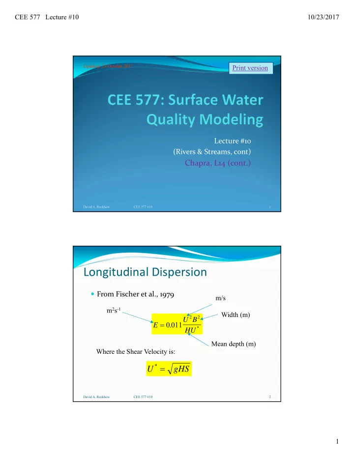
Longitudinal Dispersion

 From Fischer et al., 1979

David A. Reckhow CEE 577 #10 2

E U B HU  0 011

2 2

.

*

Where the Shear Velocity is:

U gHS

* 

m2s-1 m/s Width (m) Mean depth (m)

CEE 577 Lecture #10 10/23/2017 2

Lateral Mixing

 Lateral or transverse dispersion coefficient for a

stream:

 Length required for complete mixing:

David A. Reckhow CEE 577 #10 3

E HU

lat  0 6

.

*

L U B E

m lat

 0 40

2

. L U B E

m lat

 010

2

.

Side discharge: Center discharge: Mean depth Shear velocity Width

General Stream Geometry

 Chapra’s nomenclature for discharge coefficients

 Velocity  Depth  Width

David A. Reckhow CEE 577 #10 4

U aQ H Q B cQ

b f

   



Where: b

f     1

Because Q=UHB

CEE 577 Lecture #10 10/23/2017 3

Sample Problem

David A. Reckhow CEE 577 #10 5

The Black River, NY between MP 74.2 and MP 64.7 is to be characterized as a constant flow - constant area reach. Assume the following cross-sectional area (Ac) were measured for the given flows:

Q (c fs ) 5 7 5 1 3 0 2 2 0 3 4 A

c

(ft2) 6 8 9 5 1 1 0 1 6 0 2 2

MP 74.2 MP 64.7 Estimate travel time through this reach for flows of 600 and 3000 cfs

Thomann & Mueller, problem 2.1

David A. Reckhow CEE 577 #10 6

) ( f f

cQ BH A cQ B Q H



   

 

 

Flow (cfs)

500 600 700 800 2000 3000 4000 5000 1000

Area, sq. ft.

500 600 700 800 2000 1000 b[0]=2.9235296469 b[1]=0.581536813 r ²=0.9788480936

589 .

3 . 18 Q A 

CEE 577 Lecture #10 10/23/2017 4

Manning Equation

 Derived from the momentum balance

 relates velocity to channel characteristics including

slope

David A. Reckhow CEE 577 #10 7

U n R Se  1486

23 12

.

ft/s Manning’s roughness coefficient 0.012-0.100 see Table 14.3 Hydraulic Radius (ft) =Ac/wetted perimenter Ac/(B+2H) Slope of energy grade line = slope of stream bed for constant H & U

Manning Equation adapted to a Trapezoidal section

 Area, perimeter and

hydraulic radius can all be expressed as a function of depth

 substitute these into the

Manning Equation and calculate “y” from known “Q

David A. Reckhow CEE 577 #10 8 2 1 3 2

486 . 1

e c

S R A n Q 

y

   

1 2 1 2

2 2

          s y B y sy B P A R s y B P y sy B A

• c
• c

   

 

2 / 1 3 / 2 2 3 / 5

1 2 486 . 1

e

• S

s y B y sy B n Q    

1 s Bo

CEE 577 Lecture #10 10/23/2017 5

Distributed Systems

 Lecture #9 in Chapra’s book

 systems that have spatial resolution

 Ideal Reactors

David A. Reckhow CEE 577 #10 9

x

H B Jin Jout

V c t J A J A reaction

in c

• ut

c

    

Plug‐Flow Reactors (PRF)

David A. Reckhow CEE 577 #10 10

V c t J A J A reaction

in c

• ut

c

    

   V c t UcA U c c x x A k Vc

c c

             

Combining and taking the limit as x0

    c t U c x kc   

Which at steady state is:

0    U c x kc  

And for c=co at x=0:

c c e

• k x u





CEE 577 Lecture #10 10/23/2017 6

Plug Flow vs CSTR

 First order reactions  Mixed Flow: intermediate

 read section 9.1.3

David A. Reckhow CEE 577 #10 11

c c e

• k x u





c c Q Q kV

• 



Mixed Flow

David A. Reckhow CEE 577 #10 12

CEE 577 Lecture #10 10/23/2017 7

Mixed Flow

 Peclet Number

David A. Reckhow CEE 577 #10 13

V c t J A J A reaction

in c

• ut

c

    

    V c t Uc E c x A U c c x x E c x x c x x A k Vc

c c

                                                

Consider mixing in the longitudinal direction

P LU E

e 

 rate of advective transport rate of dispersive transport

Pe > 10, PFR-like Pe < 0.1, CSTR-like

Application of PRF to streams

 Point sources  Mass balance:

 Water Flow  Concentration

David A. Reckhow CEE 577 #10 14

Outfall: Qwcw Qrcr Qco

Q Q Q

w r

 

c Q c Q c Q Q

• w

w r r w r

  

CEE 577 Lecture #10 10/23/2017 8

Assumptions

David A. Reckhow CEE 577 #10 15

Chloride Problem

 Determine the required industrial reduction in

chlorides to maintain a desired chloride concentration

• f 250 mg/L at the intake

David A. Reckhow CEE 577 #10 16

Q=25 cfs c=30 mg/L Qw=6.5 MGD cw = 1500 mg/L QT= 5 cfs cT = 30 mg/L Water intake

1.55 cfs/MGD

CEE 577 Lecture #10 10/23/2017 9

David A. Reckhow CEE 577 #10 17

Q s

W

x x

Q s

x+ x x+ x x+ x x

 To next lecture

David A. Reckhow CEE 577 #10 18