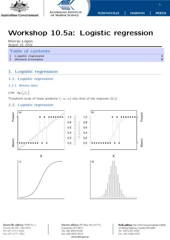
Logistic Regression Many slides attributable to: Prof. Mike Hughes - PowerPoint PPT Presentation

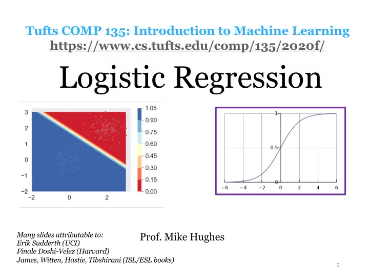
Tufts COMP 135: Introduction to Machine Learning https://www.cs.tufts.edu/comp/135/2020f/ Logistic Regression Many slides attributable to: Prof. Mike Hughes Erik Sudderth (UCI) Finale Doshi-Velez (Harvard) James, Witten, Hastie, Tibshirani (ISL/ESL books) 2

Objectives Today : Logistic Regression Logistic Regression • View as a probabilistic classifier • Justification: minimize “log loss” is equivalent to maximizing the likelihood of training set • Computing log loss in numerically stable way • Computing the gradient wrt parameters • Training via gradient descent Mike Hughes - Tufts COMP 135 - Fall 2020 3

Check-in Q1: When training Logistic Regression, we minimize the log loss on the training set. log loss( y, ˆ p ) = − y log ˆ p − (1 − y ) log(1 − ˆ p ) N X min log loss( y n , ˆ p ( x n , w, b )) w,b n =1 Can you provide 2 justifications for why this log loss objective is sensible? Mike Hughes - Tufts COMP 135 - Fall 2020 4

Check-in Q1: When training Logistic Regression, we minimize the log loss on the training set. log loss( y, ˆ p ) = − y log ˆ p − (1 − y ) log(1 − ˆ p ) N X min log loss( y n , ˆ p ( x n , w, b )) w,b n =1 Can you provide 2 justifications for why this log loss objective is sensible? 1) Log loss is an upper bound of error rate. Minimizing log loss must reduce our (worst case) error rate. 2) Log loss = Binary Cross Entropy. Interpret as learning best probabilistic “encoding’ of the training data Mike Hughes - Tufts COMP 135 - Fall 2020 5

What will we learn? Evaluation Supervised Training Learning Data, Label Pairs Performance { x n , y n } N measure Task n =1 Unsupervised Learning data label x y Reinforcement Learning Prediction Mike Hughes - Tufts COMP 135 - Fall 2020 6

Task: Binary Classification y is a binary variable Supervised (red or blue) Learning binary classification x 2 Unsupervised Learning Reinforcement Learning x 1 Mike Hughes - Tufts COMP 135 - Fall 2020 7

Probability Prediction Goal: Predict probability of label given features x i , [ x i 1 , x i 2 , . . . x if . . . x iF ] • Input: “features” Entries can be real-valued, or “covariates” other numeric types (e.g. integer, binary) “attributes” p i , p ( Y i = 1 | x i ) • Output: ˆ Value between 0 and 1 e.g. 0.001, 0.513, 0.987 “probability” >>> yproba_N2 = model. predict_proba (x_NF) >>> yproba1_N = model. predict_proba (x_NF) [:,1] >>> yproba1_N[:5] [0.143, 0.432, 0.523, 0.003, 0.994] Mike Hughes - Tufts COMP 135 - Fall 2020 8

Review: Logistic Regression Parameters: w = [ w 1 , w 2 , . . . w f . . . w F ] weight vector b bias scalar Prediction: 0 1 F X p ( y i = 1 | x i ) , sigmoid w f x if + b p ( x i , w, b ) = ˆ @ A f =1 1 sigmoid( z ) = 1 + e − z Training: Find weights and bias that minimize (penalized) log loss N X min log loss( y n , ˆ p ( x n , w, b )) w,b n =1 Mike Hughes - Tufts COMP 135 - Fall 2020 9

Logistic Regression: Predicted Probas vs Binary Decisions Predicted probability function is Decision boundary is the set of monotonically increasing in one x values where Pr(y=1|x) = 0.5 direction That direction is perpendicular Decision boundary is a linear to the decision boundary function of x Mike Hughes - Tufts COMP 135 - Fall 2020 10

Check-in (warm up for lab) Consider logistic regression classifier for 2D features What is the value (approximately) of w_1, w_2, and bias for each plot below? Predicted proba of x_2 positive class x_1 Mike Hughes - Tufts COMP 135 - Fall 2020 11

Check-in Answered Consider logistic regression classifier for 2D features What is the value (approximately) of w_1, w_2, and bias for each plot below? Predicted proba of x_2 positive class x_1 Mike Hughes - Tufts COMP 135 - Fall 2020 12

Optimization Objective Why minimize log loss? A probabilistic justification Mike Hughes - Tufts COMP 135 - Fall 2020 13

Likelihood of labels under LR We can write the probability for each possible outcome as: σ ( w T x i + b ) ⇥ p ( Y i = 1 | x i ) = σ ( w T x i + b ) ⇥ p ( Y i = 0 | x i ) = 1 − We can write the probability mass function of random variable Y as: σ ( w T x i + b ) ⇤ y i ⇥ 1 − σ ( w T x i + b ) ⇤ 1 − y i ⇥ p ( Y i = y i | x i ) = Interpret: p(y | x) is the “likelihood” of label y given input features x Goal: Fit model to make the training data as likely as possible Mike Hughes - Tufts COMP 135 - Fall 2020 14

Maximizing likelihood N Y max p ( Y n = y n | x n , w, b ) w,b n =1 Why might this be hard in practice? Hint: Think about datasets with 1000s of examples N Mike Hughes - Tufts COMP 135 - Fall 2020 15

Maximizing log likelihood The logarithm (with any base) is a monotonic transform a > b implies log (a) > log (b) Thus, the following are equivalent problems N w ∗ , b ∗ = arg max Y p ( Y n = y n | x n , w, b ) w,b n =1 " N # w ∗ , b ∗ = arg max Y log p ( Y n = y n | x n , w, b ) w,b n =1 Mike Hughes - Tufts COMP 135 - Fall 2020 16

Log likelihood for LR We can write the probability mass function of Y as: σ ( w T x i + b ) ⇤ y i ⇥ 1 − σ ( w T x i + b ) ⇤ 1 − y i ⇥ p ( Y i = y i | x i ) = Y Our training objective is to maximize log likelihood n =1 " N # w ∗ , b ∗ = arg max Y log p ( Y n = y n | x n , w, b ) w,b n =1 Mike Hughes - Tufts COMP 135 - Fall 2020 17

In order to maximize likelihood, we can minimize negative log likelihood. Two equivalent optimization problems: N w ∗ , b ∗ = arg max X log p ( Y n = y n | x n , w, b ) w,b n =1 N w ∗ , b ∗ = arg min X log p ( Y n = y n | x n , w, b ) − w,b n =1 Mike Hughes - Tufts COMP 135 - Fall 2020 18

Summary of “likelihood” justification for the way we train logistic regression • We defined a probabilistic model for y given x • We want to maximize probability of training data under this model (“maximize likelihood”) • We can show that another optimization problem (”maximize log likelihood”) is easier numerically but produces the same optimal values for weights and bias • Equivalent to minimizing -1 * log likelihood • Turns out, minimizing log loss is precisely the same thing as minimizing negative log likelihood Mike Hughes - Tufts COMP 135 - Fall 2020 19

Computing the loss for Logistic Regression (LR) in a numerically stable way Mike Hughes - Tufts COMP 135 - Fall 2020 20

<latexit sha1_base64="5EvpmrgcSyUmaOJjrly/Mlf040M=">AB/nicbVBNS8NAEN3Ur1q/quLJy2IRPJWkCnoRil48VugXtDFsNtN26WYTdjdqCQX/ihcPinj1d3jz37htc9DWBwOP92aYmefHnClt29Wbml5ZXUtv17Y2Nza3inu7jVlEgKDRrxSLZ9oAzAQ3NId2LIGEPoeWP7ye+K17kIpFoq5HMbgh6QvWY5RoI3nFA+UJfIkf7uq4qxkPIH0ce0Yv2WV7CrxInIyUIaV/zqBhFNQhCacqJUx7Fj7aZEakY5jAvdREFM6JD0oWOoICEoN52eP8bHRglwL5KmhMZT9fdESkKlRqFvOkOiB2rem4j/eZ1E9y7clIk40SDobFEv4VhHeJIFDpgEqvnIEIlM7diOiCSUG0SK5gQnPmXF0mzUnZOy5Xbs1L1Kosjw7RETpBDjpHVXSDaqiBKErRM3pFb9aT9WK9Wx+z1pyVzeyjP7A+fwB9mpUy</latexit> Simplified notation • Feature vector with first entry constant • Weight vector (first entry is the “bias”) w = [ w 0 w 1 w 2 . . . w F ] • “Score” value s (real number, -inf to +inf) s n = w T ˜ x n Mike Hughes - Tufts COMP 135 - Fall 2020 21