Linear filtering Motivation: Image denoising How can we reduce - - PowerPoint PPT Presentation

linear filtering motivation image denoising
SMART_READER_LITE
LIVE PREVIEW

Linear filtering Motivation: Image denoising How can we reduce - - PowerPoint PPT Presentation

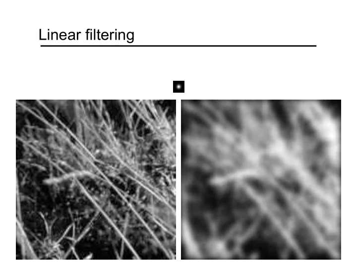
Linear filtering Motivation: Image denoising How can we reduce noise in a photograph? Moving average Lets replace each pixel with a weighted average of its neighborhood The weights are called the filter kernel What are the


slide-1
SLIDE 1

Linear filtering

slide-2
SLIDE 2

Motivation: Image denoising

  • How can we reduce noise in a photograph?
slide-3
SLIDE 3
  • Let’s replace each pixel with a weighted

average of its neighborhood

  • The weights are called the filter kernel
  • What are the weights for the average of a

3x3 neighborhood?

Moving average

1 1 1 1 1 1 1 1 1 “box filter”

Source: D. Lowe

slide-4
SLIDE 4

Defining convolution

− − = ∗

l k

l k g l n k m f n m g f

,

] , [ ] , [ ] , )[ (

f

  • Let f be the image and g be the kernel. The
  • utput of convolving f with g is denoted f * g.

Source: F. Durand

  • MATLAB functions: conv2, filter2, imfilter

Convention: kernel is “flipped”

slide-5
SLIDE 5

Key properties

  • Linearity: filter(f1 + f2) = filter(f1) + filter(f2)
  • Shift invariance: same behavior regardless of

pixel location: filter(shift(f)) = shift(filter(f))

  • Theoretical result: any linear shift-invariant
  • perator can be represented as a convolution
slide-6
SLIDE 6

Properties in more detail

  • Commutative: a * b = b * a
  • Conceptually no difference between filter and signal
  • Associative: a * (b * c) = (a * b) * c
  • Often apply several filters one after another: (((a * b1) * b2) * b3)
  • This is equivalent to applying one filter: a * (b1 * b2 * b3)
  • Distributes over addition: a * (b + c) = (a * b) + (a * c)
  • Scalars factor out: ka * b = a * kb = k (a * b)
  • Identity: unit impulse e = […, 0, 0, 1, 0, 0, …],

a * e = a

slide-7
SLIDE 7

Dealing with edges

What is the size of the output?

  • MATLAB: filter2(g, f, shape)
  • shape = ‘full’: output size is sum of sizes of f and g
  • shape = ‘same’: output size is same as f
  • shape = ‘valid’: output size is difference of sizes of f and g

f g g g g f g g g g f g g g g full same valid

slide-8
SLIDE 8

Dealing with edges

What about missing pixel values?

  • the filter window falls off the edge of the image
  • need to extrapolate
  • methods:

– clip filter (black) – wrap around – copy edge – reflect across edge

Source: S. Marschner

slide-9
SLIDE 9

Dealing with edges

What about missing pixel values?

  • the filter window falls off the edge of the image
  • need to extrapolate
  • methods (MATLAB):

– clip filter (black): imfilter(f, g, 0) – wrap around: imfilter(f, g, ‘circular’) – copy edge: imfilter(f, g, ‘replicate’) – reflect across edge: imfilter(f, g, ‘symmetric’)

Source: S. Marschner

slide-10
SLIDE 10

Practice with linear filters

1 Original

?

Source: D. Lowe

slide-11
SLIDE 11

Practice with linear filters

1 Original Filtered (no change)

Source: D. Lowe

slide-12
SLIDE 12

Practice with linear filters

1 Original

?

Source: D. Lowe

slide-13
SLIDE 13

Practice with linear filters

1 Original Shifted left By 1 pixel

Source: D. Lowe

slide-14
SLIDE 14

Practice with linear filters

Original

?

1 1 1 1 1 1 1 1 1

Source: D. Lowe

slide-15
SLIDE 15

Practice with linear filters

Original 1 1 1 1 1 1 1 1 1 Blur (with a box filter)

Source: D. Lowe

slide-16
SLIDE 16

Practice with linear filters

Original 1 1 1 1 1 1 1 1 1 2

  • ?

(Note that filter sums to 1)

Source: D. Lowe

slide-17
SLIDE 17

Practice with linear filters

Original 1 1 1 1 1 1 1 1 1 2

  • Sharpening filter
  • Accentuates differences

with local average

Source: D. Lowe

slide-18
SLIDE 18

Sharpening

Source: D. Lowe

slide-19
SLIDE 19

Sharpening

What does blurring take away?

  • riginal

smoothed (5x5)

detail

=

sharpened

=

Let’s add it back:

  • riginal

detail

+

slide-20
SLIDE 20

Smoothing with box filter revisited

  • What’s wrong with this picture?
  • What’s the solution?

Source: D. Forsyth

slide-21
SLIDE 21

Smoothing with box filter revisited

  • What’s wrong with this picture?
  • What’s the solution?
  • To eliminate edge effects, weight contribution of

neighborhood pixels according to their closeness to the center “fuzzy blob”

slide-22
SLIDE 22

Gaussian Kernel

  • Constant factor at front makes volume sum to 1 (can be

ignored when computing the filter values, as we should renormalize weights to sum to 1 in any case)

0.003 0.013 0.022 0.013 0.003 0.013 0.059 0.097 0.059 0.013 0.022 0.097 0.159 0.097 0.022 0.013 0.059 0.097 0.059 0.013 0.003 0.013 0.022 0.013 0.003

5 x 5, σ = 1

Source: C. Rasmussen

slide-23
SLIDE 23

Gaussian Kernel

  • Standard deviation σ: determines extent of smoothing

Source: K. Grauman

σ = 2 with 30 x 30 kernel σ = 5 with 30 x 30 kernel

slide-24
SLIDE 24

Choosing kernel width

  • The Gaussian function has infinite support,

but discrete filters use finite kernels

Source: K. Grauman

slide-25
SLIDE 25

Choosing kernel width

  • Rule of thumb: set filter half-width to about 3σ
slide-26
SLIDE 26

Gaussian vs. box filtering

slide-27
SLIDE 27

Gaussian filters

  • Remove high-frequency components from the

image (low-pass filter)

  • Convolution with self is another Gaussian
  • So can smooth with small-σ kernel, repeat, and get same

result as larger-σ kernel would have

  • Convolving two times with Gaussian kernel with std. dev. σ

is same as convolving once with kernel with std. dev.

  • Separable kernel
  • Factors into product of two 1D Gaussians
  • Discrete example:

Source: K. Grauman

2 σ

[ ]

1 2 1 1 2 1 1 2 1 2 4 2 1 2 1 ⎥ ⎥ ⎥ ⎦ ⎤ ⎢ ⎢ ⎢ ⎣ ⎡ = ⎥ ⎥ ⎥ ⎦ ⎤ ⎢ ⎢ ⎢ ⎣ ⎡

slide-28
SLIDE 28

Separability of the Gaussian filter

Source: D. Lowe

slide-29
SLIDE 29

Why is separability useful?

  • Separability means that a 2D convolution can

be reduced to two 1D convolutions (one among rows and one among columns)

  • What is the complexity of filtering an n×n

image with an m×m kernel?

  • O(n2 m2)
  • What if the kernel is separable?
  • O(n2 m)
slide-30
SLIDE 30

Noise

  • Salt and pepper

noise: contains random occurrences

  • f black and white

pixels

  • Impulse noise:

contains random

  • ccurrences of white

pixels

  • Gaussian noise:

variations in intensity drawn from a Gaussian normal distribution

Source: S. Seitz

slide-31
SLIDE 31

Gaussian noise

  • Mathematical model: sum of many

independent factors

  • Good for small standard deviations
  • Assumption: independent, zero-mean noise

Source: M. Hebert

slide-32
SLIDE 32

Smoothing with larger standard deviations suppresses noise, but also blurs the image

Reducing Gaussian noise

slide-33
SLIDE 33

Reducing salt-and-pepper noise

What’s wrong with the results?

3x3 5x5 7x7

slide-34
SLIDE 34

Alternative idea: Median filtering

  • A median filter operates over a window by

selecting the median intensity in the window

  • Is median filtering linear?

Source: K. Grauman

slide-35
SLIDE 35

Median filter

  • Is median filtering linear?
  • Let’s try filtering

1 1 1 1 1 2 2 2 2 ! " # # # $ % & & & + 1 ! " # # # $ % & & &

slide-36
SLIDE 36

Median filter

  • What advantage does median filtering have
  • ver Gaussian filtering?
  • Robustness to outliers

Source: K. Grauman

slide-37
SLIDE 37

Median filter

Salt-and-pepper noise Median filtered

Source: M. Hebert

MATLAB: medfilt2(image, [h w])

slide-38
SLIDE 38

Gaussian vs. median filtering

3x3 5x5 7x7 Gaussian Median

slide-39
SLIDE 39

Review: Image filtering

  • Convolution
  • Image smoothing
  • Gaussian filter
  • Nonlinear filtering
slide-40
SLIDE 40

Sharpening revisited

Source: D. Lowe

slide-41
SLIDE 41

Sharpening revisited

What does blurring take away?

  • riginal

smoothed (5x5)

detail

=

sharpened

=

Let’s add it back:

  • riginal

detail

+ α

slide-42
SLIDE 42

Unsharp mask filter

Gaussian unit impulse Laplacian of Gaussian

) ) 1 (( ) 1 ( ) ( g e f g f f g f f f − + ∗ = ∗ − + = ∗ − + α α α α

image blurred image unit impulse (identity)

slide-43
SLIDE 43

Application: Hybrid Images

  • A. Oliva, A. Torralba, P.G. Schyns,

“Hybrid Images,” SIGGRAPH 2006

slide-44
SLIDE 44
slide-45
SLIDE 45

Application: Hybrid Images

  • A. Oliva, A. Torralba, P.G. Schyns,

“Hybrid Images,” SIGGRAPH 2006

Gaussian Filter Laplacian Filter