Linear Classifier Linear classifiers are single layer neural - - PowerPoint PPT Presentation

Linear Classifier

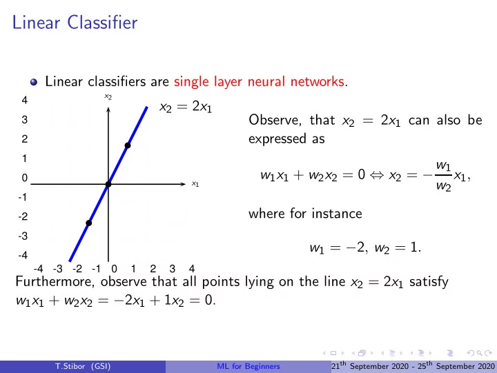
Linear classifiers are single layer neural networks.

• 4
• 3
• 2
• 1

1 2 3 4

• 4
• 3
• 2
• 1

1 2 3 4

x2 = 2x1

x1 x2

b b b

Observe, that x2 = 2x1 can also be expressed as w1x1 + w2x2 = 0 ⇔ x2 = −w1 w2 x1, where for instance w1 = −2, w2 = 1. Furthermore, observe that all points lying on the line x2 = 2x1 satisfy w1x1 + w2x2 = −2x1 + 1x2 = 0.

T.Stibor (GSI) ML for Beginners 21th September 2020 - 25th September 2020

Linear Classifier & Dot Product

• 4
• 3
• 2
• 1

1 2 3 4

• 4
• 3
• 2
• 1

1 2 3 4

−2x1 + 1x2 = 0

x1 x2

w

b

x = (1, 2)

What about the vector w = (w1, w2) = (−2, 1)? Vector w is perpendicular to the line −2x1 + 1x2 = 0. Let us calculate the dot product of w and x. The dot product is defined as w1x1 + w2x2 + . . . + wdxd = wT · x def = w, x, for some d ∈ N. In our example d = 2 and we obtain −2 · 1 + 1 · 2 = 0.

T.Stibor (GSI) ML for Beginners 21th September 2020 - 25th September 2020

Linear Classifier & Dot Product (cont.)

Let us consider the weight vector w = (3, 0) and vector x = (2, 2).

• 4
• 3
• 2
• 1

1 2 3 4

• 4
• 3
• 2
• 1

1 2 3 4

3x1 + 0x2 = 0

x1 x2

w

b

x = (2, 2)

w,x w = 3·2+0·2 √ 32

= 2 Geometric interpretation of the dot product: Length of the projection of x

• nto the unit vector w/w.

T.Stibor (GSI) ML for Beginners 21th September 2020 - 25th September 2020

Dot Product as a Similarity Measure

Dot product allows us to compute: lengths, angles and distances. Length (norm): x = x1x1 + x2x2 + . . . + xdxd = x, x Example: x = (1, 1, 1) we obtain x = √ 12 + 12 + 12 = √ 3 Angle: cos α = w, x wx = w1x1 + w2x2 + . . . + wdxd

• w2

1 + w2 2 + . . . + w2 d

• x2

1 + x2 2 + . . . + x2 d

Example: w = (3, 0), x = (2, 2) we obtain cos α = w, x wx = 3 · 2 + 0 · 2 √ 32 + 02√ 22 + 22 = 2 √ 8 and obtain α = cos−1

2 √ 8

• = 0.7853982 and 0.7853982 · 180/π = 45◦

T.Stibor (GSI) ML for Beginners 21th September 2020 - 25th September 2020

Dot Product as a Similarity Measure (cont.)

Distance (Euclidean): dist(w, x) = w − x =

• w − x, w − x =
• (w1 − x1)2 + (w2 − x2)2

Example: w = (3, 0), x = (2, 2) we obtain w − x =

• w − x, w − x =
• (3 − 2)2 + (0 − 2)2 =

√ 5 Popular application in natural language processing: Dot product on text documents, in other words how similar are e.g. two given text documents.

T.Stibor (GSI) ML for Beginners 21th September 2020 - 25th September 2020

Linear Classifier & Two Half-Spaces

• 4
• 3
• 2
• 1

1 2 3 4

• 4
• 3
• 2
• 1

1 2 3 4

{x| − 2x1 + 1x2 = 0} {x| − 2x1 + 1x2 < 0} {x| − 2x1 + 1x2 > 0} x1 x2

w

b b b b b

The x-space is separated in two half-spaces.

T.Stibor (GSI) ML for Beginners 21th September 2020 - 25th September 2020

Linear Classifier & Dot Product (cont.)

Observe, that w1x1 + w2x2 = 0 implies, that the separating line always goes through the origin. By adding an offset (bias), that is w0 + w1x1 + w2x2 = 0 ⇔ x2 = − w1

w2x1 − w0 w2 ≡ y = mx + b, one can

shift the line arbitrary.

• 4
• 3
• 2
• 1

1 2 3 4

• 4
• 3
• 2
• 1

1 2 3 4

x1 x2 w0 + w1x1 + w2x2 = 0

• 4
• 3
• 2
• 1

1 2 3 4

• 4
• 3
• 2
• 1

1 2 3 4

x1 x2 w0 + w1x1 + w2x2 > threshold T.Stibor (GSI) ML for Beginners 21th September 2020 - 25th September 2020

Linear Classifier & Single Layer NN

x0 x1 xd x1 w0 w1 wd

b b b b b

Input Output f (x)

⇔

• 4
• 3
• 2
• 1

1 2 3 4

• 4
• 3
• 2
• 1

1 2 3 4

x1 x2

Note that x0 = 1, f (x) = w, x. Given data which we want to separate, that is, a sample X = {(x1, y1), (x2, y2), . . . , (xN, yN)} ∈ Rd+1 × {−1, +1}. How to determine the proper values of w such that the “minus” and “plus” points are separated by f (x)? Infer the values of w from the data by some learning algorithm.

T.Stibor (GSI) ML for Beginners 21th September 2020 - 25th September 2020

Perceptron

Note, so far we have not seen a method for finding the weight vector w to

• btain a linearly separation of the training set.

Let f (a) be (sign) activation function f (a) = −1 if a < 0 +1 if a ≥ 0 and decision function f (w, x) = f d

• i=0

wixi

• .

Note: x0 is set to +1, that is, x = (1, x1, . . . , xd). Training pattern consists of (x, y) ∈ Rd+1 × {−1, +1}

T.Stibor (GSI) ML for Beginners 21th September 2020 - 25th September 2020

Perceptron Learning Algorithm

input : (x1, y1), . . . , (xN, yN) ∈ Rd+1 × {−1, +1}, η ∈ R+, max.epoch ∈ N

• utput: w

begin Randomly initialize w ; epoch ← 0 ; repeat for i ← 1 to N do if yiw, xi ≤ 0 then w ← w + ηxi yi epoch ← epoch + 1 until (epoch = max.epoch) or (no change in w); return w

T.Stibor (GSI) ML for Beginners 21th September 2020 - 25th September 2020

Training the Perceptron (cont.)

Geometrical explanation: If x belongs to {+1} and w, x < 0 ⇒ angle between x and w is greater than 90◦, rotate w in direction of x to bring missclassified x into the positive half space defined by w. Same idea if x belongs to {−1} and w, x ≥ 0.

+1 positive halfspace −1 negative halfspace x w +1 positive halfspace −1 negative halfspace x w w

new

T.Stibor (GSI) ML for Beginners 21th September 2020 - 25th September 2020

Perceptron Error Reduction

Recall: missclassifcation results in: wnew = w + ηx y, this reduces the error since1 −wT

new(x y)

= −wT(x y) − η

• >0

(x y)T (x y)

• xy2>0

< −wTxy How often one has to cycle through the patterns in the training set? A finite number of steps?

1right multiply with −(x y) and transpose term before T.Stibor (GSI) ML for Beginners 21th September 2020 - 25th September 2020

Perceptron Convergence Theorem

Proposition

Given a finite and linearly separable training set. The perceptron converges after some finite steps [Rosenblatt, 1962].

T.Stibor (GSI) ML for Beginners 21th September 2020 - 25th September 2020

Perceptron Algorithm (R-code)

################################################### perceptron <- function(w,X,y,eta,max.epoch) { ################################################### N <- nrow(X); epoch <- 0; repeat { w.old <- w; for (i in 1:N) { if ( y[i] * (X[i,] %*% w) <= 0 ) w <- w + eta * y[i] * X[i,]; } epoch <- epoch + 1; if ( identical(w.old,w) || epoch = max.epoch ) { break; # terminate if no change in weights or max.epoch } } return (w); }

T.Stibor (GSI) ML for Beginners 21th September 2020 - 25th September 2020

Perceptron Algorithm Visualization

−4 −2 2 4 6 −4 −2 2 4 6 X[, 2:3][,1] X[, 2:3][,2] −4 −2 2 4 6 −4 −2 2 4 6 X[, 2:3][,1] X[, 2:3][,2]

One epoch terminate if no change in w

T.Stibor (GSI) ML for Beginners 21th September 2020 - 25th September 2020

Perceptron Algorithm Visualization

−4 −2 2 4 6 −4 −2 2 4 6 X[, 2:3][,1] X[, 2:3][,2] −4 −2 2 4 6 −4 −2 2 4 6 X[, 2:3][,1] X[, 2:3][,2]

One epoch terminate if no change in w

T.Stibor (GSI) ML for Beginners 21th September 2020 - 25th September 2020

From Perceptron LossΘ to Gradient Descent

The parameters to learn are: (w0, w1, w2) = w. What is our loss function LossΘ we would like to minimize? Where is term wnew = w + ηx y coming from? LossΘ = E(w) = −

• m∈M

w, xmym where M denotes the set of all missclassified patterns. Moreover, LossΘ is continuous and piecewise linear and fits in the spirit iterative gradient descent method wnew = w + η∇E(w) = w + ηx y

T.Stibor (GSI) ML for Beginners 21th September 2020 - 25th September 2020

Method of Gradient Descent

Let E(w) be a continuously differentiable function of some unknown (weight) vector w. Find an optimal solution w⋆ that satisfies the condition E(w⋆) ≤ E(w). The necessary condition for optimality is ∇E(w⋆) = 0. Let us consider the following iterative descent: Start with an initial guess w(0) and generate sequence of weight vectors w(1), w(2), . . . such that E(w(i+1)) ≤ E(w(i)).

T.Stibor (GSI) ML for Beginners 21th September 2020 - 25th September 2020

Gradient Descent Algorithm

w(i+1) = w(i) − η∇E(w(i)) where η is a positive constant called learning rate. At each iteration step the algorithm applies the correction ∆w(i) = w(i+1) − w(i) = −η∇E(w(i)) Gradient descent algorithm satisfies: E(w(i+1)) ≤ E(w(i)), to see this, use first-order Taylor expansion around w(i) to approximate E(w(i+1)) as E(w(i)) + (∇E(w(i)))T ∆w(i).

T.Stibor (GSI) ML for Beginners 21th September 2020 - 25th September 2020

Gradient Descent Algorithm (cont.)

E(w(i+1)) ≈ E(w(i)) + (∇E(w(i)))T ∆w(i) = E(w(i)) − η∇E(w(i))2 For positive learning rate η, E(w(i)) decreases in each iteration step (for small enough learning rates). At minimum/saddle point gradient vector is 0, thus no change in weight. Example: f (x, y) = (3x2 + y) exp(−x2 − y 2) Partial derivatives: ∂f ∂x = −2x exp(−x2 − y 2)(3x2 + y − 3) ∂f ∂y = exp(−x2 − y 2)(−6x2y − 2y 2 + 1)

T.Stibor (GSI) ML for Beginners 21th September 2020 - 25th September 2020

Gradient Descent Algorithm (cont.)

−0.5 0.0 0.5 1.0 −2 −1 1 2 −2 −1 1 2

3 2

• 3
• 0.4

1

• 2
• 1

y

• 1

x 1

• 2

2

• 3

3 0.4 0.8

(3x2 + y) exp(−x2 − y 2)

See interactive demo.

T.Stibor (GSI) ML for Beginners 21th September 2020 - 25th September 2020

Gradient Descent Algorithm Example

Black points denote different starting values. Learning rate η is properly chosen, however for starting value (1, 1), algorithm converges not to the global minimum. It follows steepest descent in the “wrong direction”, in

• ther words, gradient based algorithms are local search algorithms.

−2 −1 1 2 −2 −1 1 2 z = (3x1

2 + x2)exp(−x1 2 − x2 2)

η = 0.25

T.Stibor (GSI) ML for Beginners 21th September 2020 - 25th September 2020

Gradient Descent Algorithm Example (cont.)

Learning rate η = 1.0 is too large, algorithm oscillates in a “zig-zag” manner or “overleap” the global minimum.

−2 −1 1 2 −2 −1 1 2 z = (3x1

2 + x2)exp(−x1 2 − x2 2)

η = 1

T.Stibor (GSI) ML for Beginners 21th September 2020 - 25th September 2020

Gradient Descent Algorithm Example (cont.)

Learning rate η = 0.005 is too small, algorithm converges “very slowly”.

−2 −1 1 2 −2 −1 1 2 z = (3x1

2 + x2)exp(−x1 2 − x2 2)

η = 0.005

T.Stibor (GSI) ML for Beginners 21th September 2020 - 25th September 2020

Momentum

Gradient descent can be very slow if η is too small, and can oscillate widely if η is too large. Idea: use fraction of the previous weight change and actual gradient term to control non-radical revisions in the updates. w(i+1) = w(i) − η∇E(w(i)) + αw(i−1), 0 ≤ α ≤ 1. Momentum: can cancel side-to-side oscillations across the error valley, can cause a faster convergence when weight updates are all in the same direction because the learning rate is amplified.

T.Stibor (GSI) ML for Beginners 21th September 2020 - 25th September 2020

Momentum Example Rosenbrock Function

Rosenbrock function f (x, y) = (1 − x)2 + 100(y − x2)2 has global minimum f (x, y) = (0, 0) at (1, 1). Momentum param. α = 0.021, learning rate η = 0.001.

−0.5 0.0 0.5 1.0 1.5 −0.5 0.0 0.5 1.0 1.5

number of iterations: 10 ,eta: 0.001 ,alpha : 0.021

minimum start

T.Stibor (GSI) ML for Beginners 21th September 2020 - 25th September 2020

Momentum Example Rosenbrock Func. (cont.)

Setting α = 0 (no momentum)

−0.5 0.0 0.5 1.0 1.5 −0.5 0.0 0.5 1.0 1.5

number of iterations: 5649 ,eta: 0.001 ,alpha : 0

minimum start

T.Stibor (GSI) ML for Beginners 21th September 2020 - 25th September 2020

Momentum Example Rosenbrock Func. (cont.)

Setting α = 0 (no momentum) and a larger learning rate η

−0.5 0.0 0.5 1.0 1.5 −0.5 0.0 0.5 1.0 1.5

number of iterations: 1071 ,eta: 0.003 ,alpha : 0

minimum start

T.Stibor (GSI) ML for Beginners 21th September 2020 - 25th September 2020

Sophisticated Gradient Descent

Note, gradient descent is the building block for much more sophisticated gradient descent methods such as RMSProp Adagrad Adadelta NAG Nadam These are leveraging adaptive learning rate η to speedup convergence. See: An overview of gradient descent optimization algorithms, S. Ruder

T.Stibor (GSI) ML for Beginners 21th September 2020 - 25th September 2020