Line Equation Explicit form: Given two points: y = m*x + k y = - - PowerPoint PPT Presentation

Line Equation

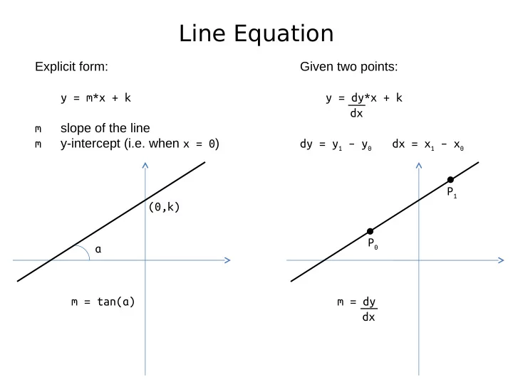
Explicit form: y = m*x + k m slope of the line m y-intercept (i.e. when x = 0) α (0,k) m = tan(α) P0 P1 Given two points: y = dy*x + k dx dy = y1 – y0 dx = x1 – x0 m = dy dx

Lines and Slopes

m = 0 (α = 0) m = +1 (α = 45) m = -1 (α = -45) m = (0..1) (α = 0..45) m = (1..∞) (α = 45..90) m = (-∞..-1) (α = -90..45) m = (-1..0) (α = -45..0) m = ∞ (α = 90)

Line Drawing (Naïve)

Given two points P0(x0,y0) and P1(x1,y1):

• 1. find the line equation y = m*x + k
• 2. for each x in [x0, x1]:

calculate y and plot (x, y) Assumptions: x0 <= x1 m = [-1..1] def drawLine(x0, y0, x1, y1): compute m and k for each x in [x0 , x1]: y = m*y + k plot(x, round(y))

Line Drawing (Incremental)

Given a line equation y = m*x + k knowing the coordinates

• f P(x,y) makes it easy to calculate y’ for the neighbor point P’(x+1,y’)

y’ = m*x’ + k = m*(x + 1) + k = m*x + m + k = m*x + k + m = y + m So to get the next y, just add the slope to the current y value def drawLine(x0, y0, x1, y1): compute the slope m start at y = y0 for each x in [x0 , x1]: plot(x, round(y)) y = y + m

Line Equation

Implicit form: a*x + b*y + c = 0 the line is all points (x,y) that satisfy the equation If we let: F(x, y) = a*x + b*y + c then F(x, y) = 0 (x,y) on the line F(x, y) < 0 (x,y) “below” the line F(x, y) > 0 (x,y) “above” the line

Line Equation

Implicit form: a*x + b*y + c = 0 the line is all points (x,y) that satisfy the equation If we let: F(x, y) = a*x + b*y + c then F(x, y) = 0 (x,y) on the line F(x, y) < 0 (x,y) “below” the line F(x, y) > 0 (x,y) “above” the line F(P) = a*x + b*y + c = 0 F(P”) = ? F(P’) = ? P” P P'

Line Equation

Implicit form: a*x + b*y + c = 0 the line is all points (x,y) that satisfy the equation If we let: F(x, y) = a*x + b*y + c then F(x, y) = 0 (x,y) on the line F(x, y) < 0 (x,y) “below” the line F(x, y) > 0 (x,y) “above” the line F(P) = a*x + b*y + c = 0 F(P”) = F(x, y+1) = a*x + b*(y+1) + c = = a*x + b*y + b + c = = a*x + b*y + c + b = = F(P) + b = b F(P’) = F(x, y-1) = -b P” P P'

Line Drawing (Midpoint)

Pick the pixel closest to the line P’ P” d” d’ Expensive, since it requires distance computation

Line Drawing (Midpoint)

Instead of calculating the true distances d’ and d” (time consuming) check on which side of the line the midpoint M lies, i.e. check whether F(M) > 0 or F(M) < 0 P’ P” d” d’ Pick P’ if M above the line, i.e. F(M) > 0 Pick P” if M is below the line, i.e. F(M) < 0 M

Line Drawing (Midpoint)

Midpoint lets us decide (1) which vertex to pick (2) which midpoint to consider next should we highlight vertex below M and move left to examine ME OR should we highlight vertex above midpoint and move diagonally to examine MNE M ? ? ME MNE

Line Drawing (Midpoint)

Midpoint lets us decide (1) which vertex to pick (2) which midpoint to consider next M ? ? M ME ? ?

Line Drawing (Midpoint)

Midpoint lets us decide (1) which vertex to pick (2) which midpoint to consider next M ? ? M MNE ? ?

Line Drawing (Midpoint)

Midpoint lets us decide (1) which vertex to pick (2) which midpoint to consider next M ? ? M ME ? ? M ? ? M MNE ? ?

Line Drawing (Midpoint)

Given two points P0(x0,y0) and P1(x1,y1) pick the closest pixels to the line. Assumptions: x0 < x1 m = [0..1] Start with the implicit equation a*x + b*y + c = 0 where a = dy, b = -dx, c = k*dx Use the idea from the incremental algorithm: if we know the value at F(M) can we calculate efficiently F(ME) or F(MNE) M ME MNE

Line Drawing (Midpoint)

Calculating the value F(ME) M ME Coordinates: M(x, y) ME(x+1,y) F(ME) = a*(x+1) + b*y + c = a*x + a + b*y + c = a*x + b*y + c + a = F(M) + a Calculating the value F(MNE) Coordinates: M(x, y) MNE(x+1,y+1) F(MNE) = a*(x+1) + b*(y+1) + c = a*x + a + b*y + b + c = a*x + b*y + c + a + b = F(M) + a + b M MNE

Line Drawing (Midpoint)

Calculating the value F(M0) Coordinates: P0(x0,y0) M0(x0+1,y0+½) F(M0) = a*(x0+1) + b*(y0+½) + c = a*x0 + a + b*y0 + b/2 + c = a*x0 + b*y0 + c + a + b/2 = F(P0) + a + b/2 = 0 + a + b/2 = a + b/2 M0 P0

Line Drawing (Midpoint)

In summary, F(Mi+1) = F(Mi) + a if Mi “above” the line, i.e. go E F(Mi+1) = F(Mi) + (a+b) if Mi “below” the line, i.e. go NE F(M0) = a + b/2 for the first midpoint M0 To avoid the division in the term b/2 we could go back and use: F(x, y) = 2a*x + 2b*y + 2c same line as F(x, y) = a*x + b*y + c Finally, F(Mi+1) = F(Mi) + 2a if Mi “above” the line, i.e. go E F(Mi+1) = F(Mi) + 2(a+b) if Mi “below” the line, i.e. go NE F(M0) = 2a + b for the first midpoint M0

Line Drawing (Issues)

Endpoint order: The assumption was that x1 < x2 i.e. drawing from “left” to “right” If x1 > x2 i.e. drawing from “right” to “left” could simply swap P1 and P2 However, swapping will not work if the lines have styles, since it will lead to discontinuities in the pattern.

Line Drawing (Issues)

Endpoint order: The assumption was that x1 < x2 i.e. drawing from “left” to “right” If x1 > x2 i.e. drawing from “right” to “left” could simply swap P1 and P2 Challenges: if lines have styles, swapping P1 and P2 will lead to discontinuities in the pattern

Line Drawing (Issues)

Starting at the edge of a clip rectangle: xmin xmax P2 P1

Line Drawing (Issues)

Starting at the edge of a clip rectangle: instead of drawLine(P1,P2) compute P'1 = (xmin, m*xmin+ k) and drawLine(P'1,P2) however, the two lines will have different slopes and will be drawn differently xmin xmax P2 P1 P'1

Line Drawing (Issues)

Starting at the edge of a clip rectangle: to fix, plot P'1 = (xmin, m*xmin+ k) but also set M0 to closest midpoint to start algo M xmin xmax P2 P1 P'1 M0

Line Drawing (Issues)

Starting at the edge of a clip rectangle: P1 P2 ymin ymax

Line Drawing (Issues)

Starting at the edge of a clip rectangle: instead of drawLine(P1,P2) compute P'1 = ((ymin-k)/m,xmin) and drawLine(P'1,P2) however, the two lines will have different slopes and will be drawn differently P1 P2 P'1 ymin ymax

Line Drawing (Issues)

Starting at the edge of a clip rectangle: may miss a pixel – adjust the clip window Ymin - ½ ymin ymax

Line Drawing (Issues)

Starting at the edge of a clip rectangle: M ymin Ymin- ½

Line Drawing (Issues)

Varying intensity with respect to slope: same number of pixels to represent different lengths