Line Characterizations Bresenhams Midpoint Algorithm y mx B - - PDF document

SLIDE 1

Spring 2013 CS5600

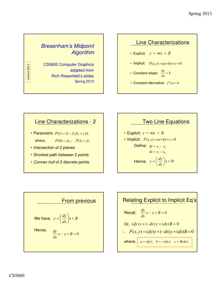
Bresenham’s Midpoint Algorithm

CS5600 Computer Graphics adapted from Rich Riesenfeld’s slides

Spring 2013

Lecture Set 2

Line Characterizations

• Explicit:
• Implicit:
• Constant slope:
• Constant derivative:

B mx y  

) , (     c by ax y x F

k x y    k x f   ) (

Line Characterizations - 2

• Parametric:

where,

• Intersection of 2 planes
• Shortest path between 2 points
• Convex hull of 2 discrete points

P t P t t P

1

) ( ) (

1

   P P P P

1

) ( ; ) (

1 



Two Line Equations

• Explicit:
• Implicit:

Define: Hence,

B mx y  

) , (     c by ax y x F

1 1

x x dx y y dy    

B x dx dy y        

From previous

We have, Hence,

B x dx dy y            B y x dx dy

Relating Explicit to Implicit Eq’s

Recall, Or, where,    B y x dx dy

) ( ) ( ) (     B dx y dx x dy

) ( ) ( ) ( ) , (       B dx y dx x dy y x F

) ( ); ( ); ( dx B c dx b dy a    

SLIDE 2

Spring 2013 CS5600

Discrete Lines

• Lines vs. Line Segments
• What is a discrete line segment?

– This is a relatively recent problem – How to generate a discrete line?

“Good” Discrete Line

• No gaps in adjacent pixels
• Pixels close to ideal line
• Consistent choices; same pixels in same situations
• Smooth looking
• Even brightness in all orientations
• Same line for as for
• Double pixels stacked up?

P P

1

P P

1

How to Draw a Line?

• 1. Compute slope
• 2. Start at on point (xo, yo)
• 3. Increment x and draw
• How to figure this out?

Derive from Line Equation

Y = mX + b Yi = mXi + b Xi+1 = Xi + X Yi+1 = mXi+1 + b Yi+1 = m(Xi+X) + b = mXi + mX + b = mX + mXi + b = mX + Yi

Derive from Line Equation

Y = mX + b Yi = mXi + b Xi+1 = Xi + X Yi+1 = mXi+1 + b Yi+1 = m(Xi+X) + b = mXi + mX + b = mX + mXi + b = mX + Yi m = y / x = (y1 – y0) / (x1 – x0) y = x (y1 – y0) / (x1 – x0) Yi+1 = Yi + Y = Yi + x (y1 – y0) / (x1 – x0) = Yi + X(m)

What about slope?

If |y1 – y0| > |x1 – x0| increment Y else increment X

SLIDE 3

Spring 2013 CS5600

CS 5600 13

• Line segment in first octant with

0 < m < 1

• After we derive this, we’ll look at the
• ther cases (other octants)

Restricted Form Incremental Fn Eval

• Recall
• Characteristics

– Fast – Cumulative Error

• Need to define

) ( ) ( ) 1 ( i x i x f i x f     ) (

• x

f

Investigate Sign of F

Verify that Look at extreme values of y

        ) , ( y x F

above line below line

• n line

The Picture

x

y

) , (  y x F

above line below line

) , (  y x F

Key to Bresenham Algorithm

“Reasonable assumptions” have reduced the problem to making a binary choice at each pixel:

(Previous) NE (next) E (next)

Decision Variable d (logical)

Define a logical decision variable d

– linear in form – incrementally updated (with addition) – tells us whether to go E or NE

SLIDE 4

Spring 2013 CS5600

The Picture

ideal line

midpoint E NE previous

Q

1  

p

x x

p

x x 

p

y y  1  

p

y y

M

The Picture (again)

ideal line

E NE

previous

Q

) , (

p p y

x ) , (

2 1

1

 

p p

y x ) 1 , 1 (  

p p

y x ) , (

1

p p

y x 

midpoint M

Observe the relationships

• Suppose Q is above M, as before.
• Then

, M is below the line

• So,

means line is above M,

• Need to move NE, increase y value

) (  M F ) (  M F

The Picture (again)

ideal line

midpoint

E NE

previous

Q

) , (

p p y

x ) , (

2 1

1

 

p p

y x ) 1 , 1 (  

p p

y x ) , (

1

p p

y x 

Observe the relationships

• Suppose Q is below M, as before.
• Then F(M) < 0 , implies M is above the

line

• So, F(M) < 0 , means line is below M,
• Need to move to E; don’t increase y

M = Midpoint = :

) , (

2 1 1

 

p p

y x

• Want to evaluate at M
• Will use an incremental

decision variable d

• Let,

) , (

2 1 1

  

p p

y x F d c y b x a d

p p

     ) ( (

2 1 ) 1

SLIDE 5

Spring 2013 CS5600

How will d be used?

Let, Therefore,

c y b x a d

p p

     ) ( (

2 1

) 1

            ) (arbitrary line) ideal above (midpoint line) ideal below (midpoint E E NE d

Case E: Suppose E is chosen

• Recall
• ...

c y b x a d

p p

• ld

     ) ( (

2 1

) 1

c y b x a y x F d

p p p p new

       



) ( ( (

2 1 2 1

) 2 ) , 2

1

: ; ,

y

E x x y    

... a d d c y b x a c y b x a d d

• ld

new p p p p

• ld

new

                         ) ( 1 ( ) ( 2 (

2 1 2 1

) )

Case E: Suppose E is chosen Review of Explicit to Implicit

Recall, Or, where,    B y x dx dy

) ( ) ( ) (     B dx y dx x dy

) ( ) ( ) ( ) , (       B dx y dx x dy y x F

) ( ); ( ); ( dx B c dx b dy a    

Case E: .

new

• ld

d d a  

increment we add if is chosen. So, . But remember that (from line equations). Hence, ( ) is not evaluated explicitly. We simply add to update for

E E E

E a a dy F M a d E       

Case NE: Suppose NE chosen

Recall ...

1 2

1)

( ( )

• ld

p p

d a x b y c     

3 2 3 2

2, ) 2)

( ( ( )

new p p p p

d F x y a x b y c        



1 1

and, : ; ,

y

NE x x y     

SLIDE 6

Spring 2013 CS5600

Case NE: Suppose NE

... b a d d c y b x a c y b x a d d

• ld

new p p p p

• ld

new

                           ) ( 1 ( ) ( 2 (

2 1 2 3

) )

Case NE: .

b a d d

• ld

new

  

increment that we add if is chosen. So, . But remember that , and (from line equations). Hence, ( ) is not evaluated explicitly. We simply add to update for

NE NE NE

NE a b a dy b dx F M a b d NE           

. for update to i.e., , add simply we means, and , where , NE d dx dy b a dx b dy a b a

NE NE NE

           

Case NE: .

b a d d

• ld

new

  

Summary

• At each step of the procedure, we

must choose between moving E or NE based on the sign of the decision variable d

• Then update according to

               dx dy d dy d d

NE NE E E

where ,

• r

, where ,

What is initial value of d ?

• First point is
• First midpoint is
• What is initial midpoint value?

) , (

0 y

x ) , (

2 1 1

  y x

) , ( ) , (

2 1 1 2 1 1

     y x F y x d  

1 1 1 1) 2 2 2 ( 2

( , ) ( ( ) , )

b b F

F x y a x b y c ax by c a x y a

 

                        

What is initial value of d ?

SLIDE 7

Spring 2013 CS5600

What is initial value of d ?

Note, ( (

, ) 0, since , ) is on line.

F x

y x y              

2 2 2 1 1

) ( ) , (

dx b

dy a y x F

Hence,

What Does Factor of 2 x Do ?

• Has the same 0-set
• Changes the slope of the plane
• Rotates plane about the 0-set line
• Gets rid of the denominator

) ( 2 ) , ( 2     c by ax y x F

1 1 2

Note, we can clear denominator and not change line, 2 ( , ) 2( ) F x y dy dx    

What is initial value of d ?

2 ( , ) 2( ) So, first value of 2( ) ( ) F x y ax by c d dy dx      

What is initial value of d ? More Summary

• Initial value
• Case E:
• Case NE:
• Note, all deltas are constants

) ( ) ( 2 dx dy  ) ( 2 where , dy d d

E E

     )} ( ) {( 2 where , dx dy d d

NE NE

     

More Summary

Choose

     

• therwise

if NE d E

SLIDE 8

Spring 2013 CS5600

Example

• Line end points:
• Deltas: dx = 4; dy = 3

) 11 , 9 ( ) , ; ) 8 , 5 ( ) ,

1 1

( (

  y x y x

Graph

13 12 11 10 9 8 7 6 4 5 6 7 8 9 10 11

Example (dx = 4; dy = 3)

• Initial value of

(5 8) 2( ) ( ) 6 4 2 2 d , dy dx d NE        

     

• therwise

if NE d E

) ( ) ( 2 dx dy 

d =

Graph

13 12 11 10 9 8 7 6 4 5 6 7 8 9 10 11

Example (dx=4; dy=3 )

• Update value of d
• Last move was NE, so

2( ) 2(3 4) 2 2 2

NE

dy - dx d           E

     

• therwise

if NE d E

) ( 2 where , dy d d

E E

     )} ( ) {( 2 where , dx dy d d

NE NE

     

Graph

13 12 11 10 9 8 7 6 4 5 6 7 8 9 10 11

SLIDE 9

Spring 2013 CS5600

Example (dx=4; dy=3 )

• Previous move was E

2( ) 2(3) 6 0 6

E dy

d NE        

     

• therwise

if NE d E

) ( 2 where , dy d d

E E

     )} ( ) {( 2 where , dx dy d d

NE NE

     

Graph

13 12 11 10 9 8 7 6 4 5 6 7 8 9 10 11

Example (dx=4; dy=3 )

• Previous move was NE

2( ) 2(3 4) 2 6 2 4

NE

dy - dx d           NE

     

• therwise

if NE d E

) ( 2 where , dy d d

E E

     )} ( ) {( 2 where , dx dy d d

NE NE

     

Graph

13 12 11 10 9 8 7 6 4 5 6 7 8 9 10 11

Graph

13 12 11 10 9 8 7 6 4 5 6 7 8 9 10 11

Meeting Bresenham Criteria

1 flip about -axis m x      1 flip about m x y     0; 1 trivial cases m m    

Case 0: Case 1: Case 2:

SLIDE 10

Spring 2013 CS5600

Case 0: Trivial Situations

• Do not need Bresenham

line horizontal    m x y m     line 1

Case 2: Flip about x-axis

) ,

(

y

x

x

y

) , 1

1

(

y

x

) , 1

1

(

y

x





) ,

(

y

x





Case 2: Flip about x-axis

Flip about -axis ( ) : x y y



  

1 1

1 1

, ) ( , , ) , )

( ); ( (

x y x y x y x y



       1

Suppose, 0 , m



  

How do slopes relate?

1 1

1 1

; by definition

y y y y

m x x m x x

 

 

 

         

) 1

( 1 i i

Since ,

y y

m y y x x



 

 

   

How do slopes relate?

) 1

1

( y y

m x x m m





    1 1       



m m

i.e.,

Case 3: Flip about line y=x

) , 1

1

(

y

x





) ,

(

y

x





y x

x

y 

) , 1

1

(

y

x

) ,

(

y

x

SLIDE 11

Spring 2013 CS5600

Case 3: Flip about line y=x

, swap and prime them , , y mx B x y x my B my x B           

Case 3: m′=?

1 , 1 and, 1 1 y x B m m m m m                        

More Raster Line Issues

• Fat lines with multiple pixel width
• Symmetric lines
• How should end pt geometry look?
• Generating curves, e.g., circles, etc.
• Jaggies, staircase effect, aliasing...

Pixel Space

12 11 10 9 8 7 6 4 5 6 7 8 9 10

Example Example

SLIDE 12

Spring 2013 CS5600

Bresenham Circles The End Bresenham’s Algorithm

Lecture Set 2