Likelihood Methods of Inference Toss coin 6 times and get Heads - PDF document
Likelihood Methods of Inference Toss coin 6 times and get Heads twice. p is probability of getting H. Probability of getting exactly 2 heads is 15 p 2 (1 p ) 4 This function of p , is likelihood function. Definition : The likelihood function
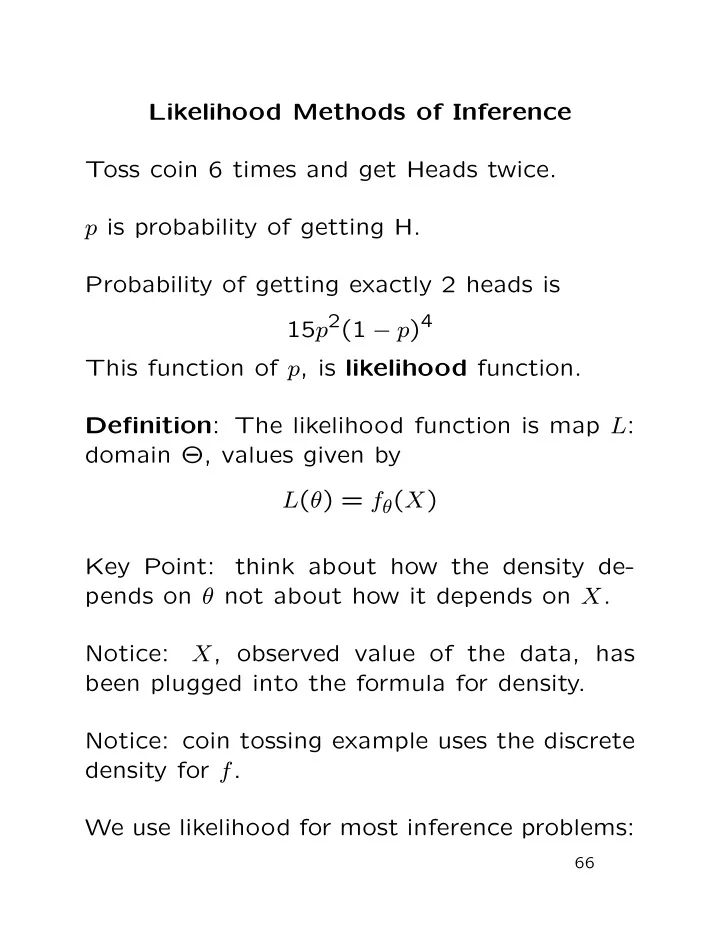
Likelihood Methods of Inference Toss coin 6 times and get Heads twice. p is probability of getting H. Probability of getting exactly 2 heads is 15 p 2 (1 − p ) 4 This function of p , is likelihood function. Definition : The likelihood function is map L : domain Θ, values given by L ( θ ) = f θ ( X ) Key Point: think about how the density de- pends on θ not about how it depends on X . Notice: X , observed value of the data, has been plugged into the formula for density. Notice: coin tossing example uses the discrete density for f . We use likelihood for most inference problems: 66
1. Point estimation: we must compute an es- timate ˆ θ = ˆ θ ( X ) which lies in Θ. The max- imum likelihood estimate (MLE) of θ is the value ˆ θ which maximizes L ( θ ) over θ ∈ Θ if such a ˆ θ exists. 2. Point estimation of a function of θ : we must compute an estimate ˆ φ = ˆ φ ( X ) of φ = g ( θ ). We use ˆ φ = g (ˆ θ ) where ˆ θ is the MLE of θ . 3. Interval (or set) estimation. We must com- pute a set C = C ( X ) in Θ which we think will contain θ 0 . We will use { θ ∈ Θ : L ( θ ) > c } for a suitable c . 4. Hypothesis testing: decide whether or not θ 0 ∈ Θ 0 where Θ 0 ⊂ Θ. We base our deci- sion on the likelihood ratio sup { L ( θ ); θ ∈ Θ 0 } sup { L ( θ ); θ ∈ Θ \ Θ 0 } 67
Maximum Likelihood Estimation To find MLE maximize L . Typical function maximization problem: Set gradient of L equal to 0 Check root is maximum, not minimum or sad- dle point. Examine some likelihood plots in examples: Cauchy Data Iid sample X 1 , . . . , X n from Cauchy( θ ) density 1 f ( x ; θ ) = π (1 + ( x − θ ) 2 ) The likelihood function is n 1 � L ( θ ) = π (1 + ( X i − θ ) 2 ) i =1 [Examine likelihood plots.] 68
Likelihood Function: Cauchy, n=5 Likelihood Function: Cauchy, n=5 1.0 1.0 0.8 0.8 0.6 0.6 Likelihood Likelihood 0.4 0.4 0.2 0.2 0.0 0.0 -10 -5 0 5 10 -10 -5 0 5 10 Theta Theta Likelihood Function: Cauchy, n=5 Likelihood Function: Cauchy, n=5 1.0 1.0 0.8 0.8 0.6 0.6 Likelihood Likelihood 0.4 0.4 0.2 0.2 0.0 0.0 -10 -5 0 5 10 -10 -5 0 5 10 Theta Theta Likelihood Function: Cauchy, n=5 Likelihood Function: Cauchy, n=5 1.0 1.0 0.8 0.8 0.6 0.6 Likelihood Likelihood 0.4 0.4 0.2 0.2 0.0 0.0 -10 -5 0 5 10 -10 -5 0 5 10 Theta Theta 69
Likelihood Function: Cauchy, n=5 Likelihood Function: Cauchy, n=5 1.0 1.0 0.8 0.8 0.6 Likelihood Likelihood 0.6 0.4 0.4 0.2 0.2 0.0 -2 -1 0 1 2 -2 -1 0 1 2 Theta Theta Likelihood Function: Cauchy, n=5 Likelihood Function: Cauchy, n=5 1.0 1.0 0.8 0.8 0.6 0.6 Likelihood Likelihood 0.4 0.4 0.2 0.2 0.0 0.0 -2 -1 0 1 2 -2 -1 0 1 2 Theta Theta Likelihood Function: Cauchy, n=5 Likelihood Function: Cauchy, n=5 1.0 1.0 0.8 0.8 0.6 0.6 Likelihood Likelihood 0.4 0.4 0.2 0.2 0.0 0.0 -2 -1 0 1 2 -2 -1 0 1 2 Theta Theta 70
Likelihood Function: Cauchy, n=25 Likelihood Function: Cauchy, n=25 1.0 1.0 0.8 0.8 0.6 0.6 Likelihood Likelihood 0.4 0.4 0.2 0.2 0.0 0.0 -10 -5 0 5 10 -10 -5 0 5 10 Theta Theta Likelihood Function: Cauchy, n=25 Likelihood Function: Cauchy, n=25 1.0 1.0 0.8 0.8 0.6 0.6 Likelihood Likelihood 0.4 0.4 0.2 0.2 0.0 0.0 -10 -5 0 5 10 -10 -5 0 5 10 Theta Theta Likelihood Function: Cauchy, n=25 Likelihood Function: Cauchy, n=25 1.0 1.0 0.8 0.8 0.6 0.6 Likelihood Likelihood 0.4 0.4 0.2 0.2 0.0 0.0 -10 -5 0 5 10 -10 -5 0 5 10 Theta Theta 71
Likelihood Function: Cauchy, n=25 Likelihood Function: Cauchy, n=25 1.0 1.0 0.8 0.8 0.6 0.6 Likelihood Likelihood 0.4 0.4 0.2 0.2 0.0 0.0 -1.0 -0.5 0.0 0.5 1.0 -1.0 -0.5 0.0 0.5 1.0 Theta Theta Likelihood Function: Cauchy, n=25 Likelihood Function: Cauchy, n=25 1.0 1.0 0.8 0.8 0.6 0.6 Likelihood Likelihood 0.4 0.4 0.2 0.2 0.0 0.0 -1.0 -0.5 0.0 0.5 1.0 -1.0 -0.5 0.0 0.5 1.0 Theta Theta Likelihood Function: Cauchy, n=25 Likelihood Function: Cauchy, n=25 1.0 1.0 0.8 0.8 0.6 0.6 Likelihood Likelihood 0.4 0.4 0.2 0.2 0.0 0.0 -1.0 -0.5 0.0 0.5 1.0 -1.0 -0.5 0.0 0.5 1.0 Theta Theta 72
I want you to notice the following points: • The likelihood functions have peaks near the true value of θ (which is 0 for the data sets I generated). • The peaks are narrower for the larger sam- ple size. • The peaks have a more regular shape for the larger value of n . • I actually plotted L ( θ ) /L (ˆ θ ) which has ex- actly the same shape as L but runs from 0 to 1 on the vertical scale. 73
To maximize this likelihood: differentiate L , set result equal to 0. Notice L is product of n terms; derivative is n 1 2( X i − θ ) � � π (1 + ( X j − θ ) 2 ) π (1 + ( X i − θ ) 2 ) 2 i =1 j � = i which is quite unpleasant. Much easier to work with logarithm of L : log of product is sum and logarithm is monotone increasing. Definition : The Log Likelihood function is ℓ ( θ ) = log { L ( θ ) } . For the Cauchy problem we have log(1 + ( X i − θ ) 2 ) − n log( π ) � ℓ ( θ ) = − [Examine log likelihood plots.] 74
Likelihood Ratio Intervals: Cauchy, n=5 Likelihood Ratio Intervals: Cauchy, n=5 -12 -10 -14 Log Likelihood Log Likelihood -15 -16 -18 -20 -20 -22 • • • • • -25 • • • • -10 -5 0 5 10 -10 -5 0 5 10 Theta Theta Likelihood Ratio Intervals: Cauchy, n=5 Likelihood Ratio Intervals: Cauchy, n=5 -5 -10 -10 Log Likelihood Log Likelihood -15 -15 -20 -20 • • • • • • • • • • -10 -5 0 5 10 -10 -5 0 5 10 Theta Theta Likelihood Ratio Intervals: Cauchy, n=5 Likelihood Ratio Intervals: Cauchy, n=5 -10 -12 -15 -14 Log Likelihood Log Likelihood -16 -18 -20 -20 -22 -25 -24 • • • • • • • • -10 -5 0 5 10 -10 -5 0 5 10 Theta Theta 75
Likelihood Ratio Intervals: Cauchy, n=5 Likelihood Ratio Intervals: Cauchy, n=5 -11.0 -8 -11.5 -12.0 Log Likelihood Log Likelihood -10 -12.5 -12 -13.0 -13.5 -14 -2 -1 0 1 2 -2 -1 0 1 2 Theta Theta Likelihood Ratio Intervals: Cauchy, n=5 Likelihood Ratio Intervals: Cauchy, n=5 -6 -2 -7 -4 -8 Log Likelihood Log Likelihood -9 -6 -10 -11 -8 -12 -2 -1 0 1 2 -2 -1 0 1 2 Theta Theta Likelihood Ratio Intervals: Cauchy, n=5 Likelihood Ratio Intervals: Cauchy, n=5 -10 -12 -11 -13 Log Likelihood Log Likelihood -14 -12 -15 -13 -16 -14 -17 -2 -1 0 1 2 -2 -1 0 1 2 Theta Theta 76
Likelihood Ratio Intervals: Cauchy, n=25 Likelihood Ratio Intervals: Cauchy, n=25 -20 -40 -40 Log Likelihood Log Likelihood -60 -60 -80 -80 -100 -100 • • • • • •• • • • • • • • • • • • • • • • • • • • • • • • • • • • • • • • • • • • • • • • • • • • -10 -5 0 5 10 -10 -5 0 5 10 Theta Theta Likelihood Ratio Intervals: Cauchy, n=25 Likelihood Ratio Intervals: Cauchy, n=25 -20 -40 -40 -60 Log Likelihood Log Likelihood -60 -80 -80 -100 -100 • • • • • • • • • • • • • • • • • • • • • • • • • • • • • • • • • • • • • • • • • • • • • • • • • • -10 -5 0 5 10 -10 -5 0 5 10 Theta Theta Likelihood Ratio Intervals: Cauchy, n=25 Likelihood Ratio Intervals: Cauchy, n=25 -40 -60 -60 Log Likelihood Log Likelihood -80 -80 -100 -100 -120 • • • • • • • • • •• • • • • •• • • • • • • • • • • • • • • • •• • • • • • • • • • • • • • -10 -5 0 5 10 -10 -5 0 5 10 Theta Theta 77
Likelihood Ratio Intervals: Cauchy, n=25 Likelihood Ratio Intervals: Cauchy, n=25 -22 -24 -24 -26 Log Likelihood Log Likelihood -26 -28 -28 -30 -30 -1.0 -0.5 0.0 0.5 1.0 -1.0 -0.5 0.0 0.5 1.0 Theta Theta Likelihood Ratio Intervals: Cauchy, n=25 Likelihood Ratio Intervals: Cauchy, n=25 -36 -22 -38 Log Likelihood Log Likelihood -24 -40 -26 -42 -28 -44 -1.0 -0.5 0.0 0.5 1.0 -1.0 -0.5 0.0 0.5 1.0 Theta Theta Likelihood Ratio Intervals: Cauchy, n=25 Likelihood Ratio Intervals: Cauchy, n=25 -43 -46 -44 -48 -45 Log Likelihood Log Likelihood -50 -46 -52 -47 -54 -48 -56 -49 -1.0 -0.5 0.0 0.5 1.0 -1.0 -0.5 0.0 0.5 1.0 Theta Theta 78
Notice the following points: • Plots of ℓ for n = 25 quite smooth, rather parabolic. • For n = 5 many local maxima and minima of ℓ . Likelihood tends to 0 as | θ | → ∞ so max of ℓ occurs at a root of ℓ ′ , derivative of ℓ wrt θ . Def’n : Score Function is gradient of ℓ U ( θ ) = ∂ℓ ∂θ MLE ˆ θ usually root of Likelihood Equations U ( θ ) = 0 In our Cauchy example we find 2( X i − θ ) � U ( θ ) = 1 + ( X i − θ ) 2 [Examine plots of score functions.] Notice: often multiple roots of likelihood equa- tions. 79
Recommend
More recommend
Explore More Topics
Stay informed with curated content and fresh updates.


