Testing: is my coin fair ? Formally: we want to make some - PDF document

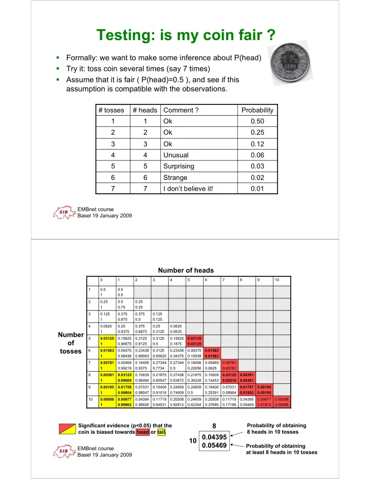
Testing: is my coin fair ? � Formally: we want to make some inference about P(head) � Try it: toss coin several times (say 7 times) � Assume that it is fair ( P(head)=0.5 ), and see if this assumption is compatible with the observations. # tosses # heads Comment ? Probability 1 1 Ok 0.50 2 2 Ok 0.25 3 3 Ok 0.12 4 4 Unusual 0.06 5 5 Surprising 0.03 6 6 Strange 0.02 7 7 I don’t believe it! 0.01 EMBnet course Basel 19 January 2009 Number of heads 0 1 2 3 4 5 6 7 8 9 10 1 0.5 0.5 1 0.5 2 0.25 0.5 0.25 1 0.75 0.25 3 0.125 0.375 0.375 0.125 1 0.875 0.5 0.125 4 0.0625 0.25 0.375 0.25 0.0625 1 0.9375 0.6875 0.3125 0.0625 Number 5 0.03125 0.15625 0.3125 0.3125 0.15625 0.03125 of 1 0.96875 0.8125 0.5 0.1875 0.03125 tosses 6 0.01563 0.09375 0.23438 0.3125 0.23438 0.09375 0.01563 1 0.98438 0.89063 0.65625 0.34375 0.10938 0.01563 7 0.00781 0.05469 0.16406 0.27344 0.27344 0.16406 0.05469 0.00781 1 0.99219 0.9375 0.7734 0.5 0.22656 0.0625 0.00781 8 0.00391 0.03125 0.10939 0.21875 0.27438 0.21875 0.10939 0.03125 0.00391 1 0.99609 0.96484 0.85547 0.63672 0.36328 0.14453 0.03516 0.00391 9 0.00195 0.01758 0.07031 0.16406 0.24609 0.24609 0.16406 0.07031 0.01757 0.00195 1 0.99804 0.98047 0.91016 0.74609 0.5 0.25391 0.08984 0.01953 0.00195 10 0.00098 0.00977 0.04394 0.11719 0.20508 0.24609 0.20508 0.11719 0.04395 0.00977 0.00098 1 0.99902 0.98926 0.94531 0.82812 0.62304 0.37695 0.17188 0.05469 0.01074 0.00098 Significant evidence (p<0.05) that the 8 Probability of obtaining coin is biased towards head or tail. 8 heads in 10 tosses 0.04395 10 0.05469 Probability of obtaining EMBnet course at least 8 heads in 10 tosses Basel 19 January 2009

Observations: taking samples � Samples are taken from an Underlying Population underlying real or fictitious population Sample 1 � Samples can be of different Sample 2 size � Samples can be overlapping Sample 3 � Samples are assumed to be taken at random and independently from each other Estimation: � Samples are assumed to be � Sample 1 => Mean 1 representative of the population (the population � Sample 2 => Mean 2 “homogeneous”) � Sample 3 => Mean 3 EMBnet course Basel 19 January 2009 Sampling variability � Say we sample from a population in order to estimate the population mean of some (numerical) variable of interest ( e.g. weight, height, number of children, etc .) We would use the sample mean as our guess for the unknown value of � the population mean � Our sample mean is very unlikely to be exactly equal to the (unknown) population mean just due to chance variation in sampling � Thus, it is useful to quantify the likely size of this chance variation (also called ‘chance error’ or ‘sampling error’, as distinct from ‘nonsampling errors’ such as bias ) If we estimate the mean multiple times from different samples, we will get � a certain distribution . EMBnet course Basel 19 January 2009

Central Limit Theorem (CLT) � The CLT says that if we – repeat the sampling process many times – compute the sample mean (or proportion) each time – make a histogram of all the means (or proportions) � then that histogram of sample means should look like the normal distribution � Of course, in practice we only get one sample from the population, we get one point of that normal distribution � The CLT provides the basis for making confidence intervals and hypothesis tests for means � This is proven for a large family of distributions for the data that are sampled, but there are also distributions for which the CLT is not applicable EMBnet course Basel 19 January 2009 Sampling variability of the sample mean � Say the SD in the population for the variable is known to be some number σ If a sample of n individuals has been chosen ‘at random’ from the � population, then the likely size of chance error of the sample mean (called the standard error ) is SE(mean) = σ / √ n � This the typical difference to be expected if the sampling is done twice independently and the averages are compared � 4 time more data are required to half the standard error If σ is not known, you can substitute an estimate � � Some people plot the SE instead of SD on barplots EMBnet course Basel 19 January 2009

Central Limit Theorem (CLT) Sample 1 Mean 1 Sample 2 Mean 2 Sample 3 Mean 3 Sample 4 Mean 4 Sample 5 Mean 5 Normal distribution Sample 6 Mean 6 ... ... Mean : true mean of the population : σ / √ n SD Note: this is the SD of the sample mean, also called Standard Error; it is not the SD of the original population. EMBnet course Basel 19 January 2009 Hypothesis testing � 2 hypotheses in competition: – H 0 : the NULL hypothesis, usually the most conservative – H 1 or H A : the alternative hypothesis, the one we are actually interested in. � Examples of NULL hypothesis: – The coin is fair – This new drug is no better (or worse) than a placebo – There is no difference in weight between two given strains of mice � Examples of Alternative hypothesis: – The coin is biased (either towards tail or head) – The coin is biased towards tail – The coin has probability 0.6 of landing on tail – The drug is better than a placebo EMBnet course Basel 19 January 2009

Hypothesis testing � We need something to measure how far my observation is from what I expect to see if H 0 is correct: a test statistic – Example: number of heads obtained when tossing my coin a given number of times: Low value of the test statistic � more likely not to reject H 0 High value of the test statistic � more likely to reject H 0 � Finally, we need a formal way to determine if the test statistic is “low” or “high” and actually make a decision. � We can never prove that the alternative hypothesis is true; we can only show evidence for or against the null hypothesis ! EMBnet course Basel 19 January 2009 Significance level The p-value is the probability of getting a test result that is as or more � extreme than the observed value of the test statistic. � If the distribution of the test statistic is known, a p-value can be calculated. � Historically: – A predefined significance level ( α ) is defined (typically 0.05 or 0.01) – The value of the test statistic which correspond to the significance level is calculated (usually using tables) – If the observed test statistic is above the threshold, we reject the NULL hypothesis. � Computers can now calculate exact p-values, which are reported � “p<0.05” remains a magical threshold � Confusion about p-values: – It is not the probability that the null hypothesis is correct. – It is not the probability of making an error EMBnet course Basel 19 January 2009

Hypothesis testing � How is my test statistic distributed if H 0 is correct ? P(Heads <= 1) = 0.01074 P(Heads >= 9) = 0.01074 EMBnet course Basel 19 January 2009 One-sided vs two-sided test � The choice alternative hypothesis influence the result of the test � If H A is “the coin is biased”, we do not specify the direction of the bias and we must be ready for both alternatives (many heads or many tails) � This is a two-sided test . � If the “total” significance α is e.g. 0.05, it means we must allow α /2 (0.025) for bias towards tail and α /2 (0.025) for bias towards head. � If H A is “the coin is biased towards heads”, we specify the direction of the bias and the test is one-sided . � Two-sided tests are usually recommended because they do not depend on some “prior information” (direction), although they are less powerful. EMBnet course Basel 19 January 2009

One-sided vs two-sided test 5% One-sided e.g. H A : μ >0 2.5% Two-sided 2.5% e.g. H A : μ =0 EMBnet course Basel 19 January 2009 Errors in hypothesis testing Decision not rejected rejected Truth negative positive ☺ X H 0 is true specificity Type I error False Positive α True negative TN X ☺ Power 1 - β ; Type II error H 0 is false sensitivity False Negative β True Positive TP EMBnet course Basel 19 January 2009

Power � Not only do you want to have a low FALSE positive rate, but you would also like to have a high TRUE positive rate – that is, high power , the chance to find an effect (or difference) if it is really there � Statistical tests will not be able to detect a true difference if the sample size is too small compared to the effect size of interest � To compute or estimate power of a study, you need to be able to specify the α level of the test, the sample size n , the effect size δ , and the SD σ (or an estimate s ) � In some types of studies, such as microarryas, it is difficult (impossible?) to estimate power, because not all of these quantities are typically known, and will also vary across genes ( e.g . different genes have differing amounts of variability) EMBnet course Basel 19 January 2009 One sample t-test � Is the mean of a population equal to a given value ? � Example: – Given a gene and several replicate microarray measurements (log ratios) g 1 , g 2 , …, g n . Is the gene diffentially expressed or, equivalently, is the mean of the measurements different from to 0 ? � Hypotheses: – H 0 : mean equals μ 0 (a given value, often 0) – H A : could be for example • mean different from μ 0 • mean larger than μ 0 • mean equals μ 1 (another given value) EMBnet course Basel 19 January 2009