[PPT] - Lectures 6 & 7: Optimization and Optimization and Lectures 6 PowerPoint Presentation

SLIDE 1

Ω

Lectures 6 & 7: Lectures 6 & 7: Optimization and Optimization and Uncertainty of Supply Chain Uncertainty of Supply Chain Network (2) Network (2)

Quality Assurance in Supply Chain Management (INSE 6300/4-UU) Winter 2011

Ω

INSE 6300/4 INSE 6300/4-

UU

UU

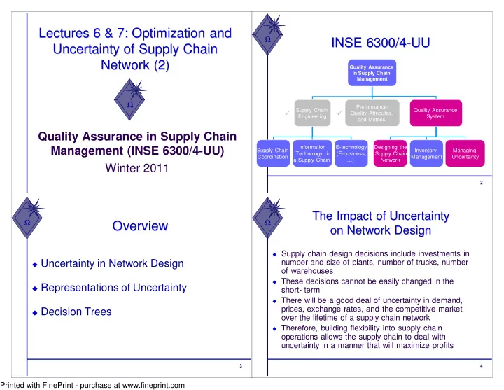
Quality Assurance In Supply Chain Management Supply Chain Engineering Performance, Quality Attributes, and Metrics Quality Assurance System Designing the Supply Chain Network Inventory Management Supply Chain Coordination Information Technology in a Supply Chain E-technology (E-business, …) Managing Uncertainty

Ω

Overview Overview

Uncertainty in Network Design Representations of Uncertainty Decision Trees

Ω

The Impact of Uncertainty The Impact of Uncertainty

n Network Design
n Network Design

Supply chain design decisions include investments in

number and size of plants, number of trucks, number

f warehouses

These decisions cannot be easily changed in the

short- term

There will be a good deal of uncertainty in demand,

prices, exchange rates, and the competitive market

ver the lifetime of a supply chain network

Therefore, building flexibility into supply chain

perations allows the supply chain to deal with

uncertainty in a manner that will maximize profits Printed with FinePrint - purchase at www.fineprint.com

SLIDE 2

Ω

Discounted Cash Flow Analysis Discounted Cash Flow Analysis

Supply chain decisions are in place for a long

time, so they should be evaluated as a sequence of cash flows over that period

Discounted cash flow (DCF) analysis

evaluates the present value of any stream of future cash flows and allows managers to compare different cash flow streams in terms

f their financial value

Based on the time value of money – a dollar

today is worth more than a dollar tomorrow

Ω

Discounted Cash Flow Analysis Discounted Cash Flow Analysis

Compare NPV of different supply chain design options

The option with the highest NPV will provide the greatest

financial return return

f

rate flows cash

f

stream this

f

lue present va net the periods T

ver

flows cash

f

stream a is ,..., , where 1 1 1 1 factor Discount

1 1

= =

+

+ = + =

=

k NPV C C C C k C NPV k

T T t t t

Ω

NPV Example: Trips Logistics NPV Example: Trips Logistics

How much space to lease in the next three years Demand = 100,000 units Requires 1,000 sq. ft. of space for every 1,000 units

f demand

Revenue = $1.22 per unit of demand Decision is whether to sign a three-year lease or

btain warehousing space on the spot market

Three-year lease: cost = $1 per sq. ft. Spot market: cost = $1.20 per sq. ft. k = 0.1

Ω

NPV Example: Trips Logistics NPV Example: Trips Logistics

For leasing warehouse space on the spot market: Expected annual profit = 100,000 x $1.22 – 100,000 x $1.20 = $2,000 Cash flow = $2,000 in each of the next three years ( )

471 , 5 $ 1 . 1 2000 1 . 1 2000 2000 1 1 lease) (no

2 2 2 1

= + + = + + + + = k C k C C NPV

Printed with FinePrint - purchase at www.fineprint.com

SLIDE 3

Ω

NPV Example: Trips Logistics NPV Example: Trips Logistics

For leasing warehouse space with a three-year lease: Expected annual profit = 100,000 x $1.22 – 100,000 x $1.00 = $22,000 Cash flow = $22,000 in each of the next three years ( )

182 , 60 $ 1 . 1 22000 1 . 1 22000 22000 1 1 lease) (no

2 2 2 1

= + + = + + + + = k C k C C NPV

The NPV of signing the lease is higher; therefore, the manager decides to sign the lease However, uncertainty in demand and costs may cause the manager to rethink his decision

Ω

Overview Overview

Uncertainty in Network Design Representations of Uncertainty Decision Trees

Ω

Representations of Uncertainty Representations of Uncertainty

Binomial Representation of Uncertainty Other Representations of Uncertainty

Normal Representation Log-normal Representation

Ω

Binomial Representations Binomial Representations

f Uncertainty
f Uncertainty

When moving from one period to the next, the value of the

underlying factor (e.g., demand or price) has only two possible outcomes – up or down

The underlying factor moves up by a factor or u > 1 with

probability p, or down by a factor d < 1 with probability 1-p

Assuming a price P in period 0, for the multiplicative

binomial, the possible outcomes for the next four periods:

Period 1: Pu, Pd Period 2: Pu2, Pud, Pd2 Period 3: Pu3, Pu2d, Pud2, Pd3 Period 4: Pu4, Pu3d, Pu2d2, Pud3, Pd4

Printed with FinePrint - purchase at www.fineprint.com

SLIDE 4

Ω

Binomial Representations Binomial Representations

f Uncertainty
f Uncertainty

In general, for multiplicative binomial, period

T has all possible outcomes Putd(T-t), for t = 0,1,…,T

From state Puad(T-a) in period t, the price may

move in period t+1 to either

Pua+1d(T-a) with probability p, or Puad(T-a)+1 with probability (1-p)

Represented as the binomial tree

Ω

The Multiplicative Binomial Tree The Multiplicative Binomial Tree

Ω

Binomial Representations Binomial Representations

f Uncertainty
f Uncertainty

For the additive binomial, the states in the

following periods are:

Period 1: P+u, P-d Period 2: P+2u, P+u-d, P-2d Period 3: P+3u, P+2u-d, P+u-2d, P-3d Period 4: P+4u, P+3u-d, P+2u-2d, P+u-3d, P-4d

In general, for the additive binomial, period T

has all possible outcomes P+tu-(T-t)d, for t=0, 1, …, T

Ω

Binomial and Normal Binomial and Normal Approximation Approximation

Printed with FinePrint - purchase at www.fineprint.com

SLIDE 5

Ω

The Normal Distribution The Normal Distribution

Ω

The Log The Log-

normal Distribution

normal Distribution

Ω

Overview Overview

Uncertainty in Network Design Representations of Uncertainty Decision Trees

Ω

Evaluating Network Design Decisions Evaluating Network Design Decisions Using Decision Trees Using Decision Trees

A manager must make many different decisions when

designing a supply chain network

Many of them involve a choice between a long-term (or less

flexible) option and a short-term (or more flexible) option

If uncertainty is ignored, the long-term option will almost always

be selected because it is typically cheaper

Such a decision can eventually hurt the firm, however, because

actual future prices or demand may be different from what was forecast at the time of the decision

A decision tree is a graphic device that can be used to

evaluate decisions under uncertainty Printed with FinePrint - purchase at www.fineprint.com

SLIDE 6

Ω

Decision Tree Methodology Decision Tree Methodology

1. Identify the duration of each period and the

number of periods T over the which the decision is to be evaluated

2. Identify factors such as demand, price, and

exchange rate, whose fluctuation will be considered over the next T periods

3. Identify representations of uncertainty for each

factor; that is, determine what distribution to use to model the uncertainty

4. Identify the periodic discount rate k for each

period

Ω

Decision Tree Methodology Decision Tree Methodology

5.

Represent the decision tree with defined states in each period, as well as the transition probabilities between states in successive periods

6.

Starting at period T, work back to period 0, identifying the optimal decision and the expected cash flows at each step. Expected cash flows at each state in a given period should be discounted back when included in the previous period

Ω

Decision Tree Methodology: Decision Tree Methodology: Trips Logistics Trips Logistics

Decide whether to lease warehouse space for the coming

three years and the quantity to lease

Long-term lease is currently cheaper than the spot market

rate

The manager anticipates uncertainty in demand and spot

prices over the next three years

Long-term lease is cheaper but could go unused if

demand is lower than forecast; future spot market rates could also decrease

Spot market rates are currently high, and the spot market

would cost a lot if future demand is higher than expected

Ω

Trips Logistics: Three Options Trips Logistics: Three Options

Get all warehousing space from the spot

market as needed

Sign a three-year lease for a fixed amount of

warehouse space and get additional requirements from the spot market

Sign a flexible lease with a minimum charge

that allows variable usage of warehouse space up to a limit with additional requirement from the spot market

Printed with FinePrint - purchase at www.fineprint.com

SLIDE 7

Ω

Trips Logistics Trips Logistics

1000 sq. ft. of warehouse space needed for 1000 units of

demand

Current demand = 100,000 units per year Binomial uncertainty: Demand can go up by 20% with

p = 0.5 or down by 20% with 1-p = 0.5

Lease price = $1.00 per sq. ft. per year Spot market price = $1.20 per sq. ft. per year Spot prices can go up by 10% with p = 0.5 or down by

10% with 1-p = 0.5

Revenue = $1.22 per unit of demand k = 0.1

Ω

Trips Logistics Decision Tree Trips Logistics Decision Tree

D=144 p=$1.45 D=144 p=$1.19 D=96 p=$1.45 D=144 p=$0.97 D=96 p=$1.19 D=96 p=$0.97 D=64 p=$1.45 D=64 p=$1.19 D=64 p=$0.97 D=120 p=$1.32 D=120 p=$1. 08 D=80 p=$1.32 D=80 p=$1.08 D=100 p=$1.20

0.25 0.25 0.25 0.25 0.25 0.25 0.25 0.25 Period 0 Period 1 Period 2

1 2 3 4 5 6 7 8 9

Ω

Trips Logistics Example Trips Logistics Example

Analyze the option of not signing a lease and

btaining all warehouse space from the spot market

Start with Period 2 and calculate the profit at each

node

For D=144, p=$1.45, in Period 2:

C(D=144, p=1.45, 2) = 144,000x1.45 = $208,800 P(D=144, p =1.45, 2) = 144,000x1.22 – C(D=144,p=1.45, 2) = 175,680-208,800 = -$33,120

Profit at other nodes:

Ω

Profit at Other Nodes Profit at Other Nodes

Printed with FinePrint - purchase at www.fineprint.com

SLIDE 8

Ω

Trips Logistics Example Trips Logistics Example

Expected profit at each node in Period 1 is the profit

during Period 1 plus the present value (in period 1) of the expected profit in Period 2

Expected profit EP(D=, p=,1) at a node is the

expected profit over all four nodes in Period 2 that may result from this node

PVEP(D=,p=,1) is the present value of this expected

profit

P(D=,p=,1), the total expected profit, is the sum of the

profit in Period 1 and the present value of the expected profit in Period 2

Ω

Trips Logistics Example Trips Logistics Example

From node D=120, p=$1.32 in Period 1, there are

four possible states in Period 2

Evaluate the expected profit in Period 2 over all four

states possible from node D=120, p=$1.32 in Period 1 to be

EP(D=120,p=1.32,1) = 0.25xP(D=144,p=1.45,2) + 0.25xP(D=144,p=1.19,2) + 0.25xP(D=96,p=1.45,2) + 0.25xP(D=96,p=1.19,2) = 0.25x(-33,120)+0.25x4,320+0.25x(-22,080)+0.25x2,880 = -$12,000

Ω

Trips Logistics Example Trips Logistics Example

The present value of this expected value in Period 1 is

PVEP(D=120, p=1.32,1) = EP(D=120,p=1.32,1) / (1+k) = -$12,000 / (1+0.1) = -$10,909

The total expected profit P(D=120,p=1.32,1) at node

D=120,p=1.32 in Period 1 is the sum of the profit in Period 1 at this node, plus the present value of future expected profits possible from this node P(D=120,p=1.32,1) = [(120,000x1.22)-(120,000x1.32)] + PVEP(D=120,p=1.32,1) = -$12,000 + (-$10,909) = -$22,909

The total expected profit for the other nodes in Period 1:

Ω

The Total Expected Profit for the The Total Expected Profit for the Other Nodes in Period 1 Other Nodes in Period 1

Printed with FinePrint - purchase at www.fineprint.com

SLIDE 9

Ω

Trips Logistics Example Trips Logistics Example

For Period 0, the total profit P(D=100,p=120,0) is the sum of the

profit in Period 0 and the present value of the expected profit

ver the four nodes in Period 1

EP(D=100,p=1.20,0) = 0.25xP(D=120,p=1.32,1) + = 0.25xP(D=120,p=1.08,1) + = 0.25xP(D=96,p=1.32,1) + = 0.25xP(D=96,p=1.08,1) = 0.25x(-22,909)+0.25x32,073+0.25x(-15,273)+0.25x21,382 = $3,818 PVEP(D=100,p=1.20,0) = EP(D=100,p=1.20,0) / (1+k) = $3,818 / (1 + 0.1) = $3,471

Ω

Trips Logistics Example Trips Logistics Example

P(D=100,p=1.20,0) = 100,000x1.22- 100,000x1.20 + PVEP(D=100,p=1.20,0) = $2,000 + $3,471 = $5,471

Therefore, the expected NPV of not signing

the lease and obtaining all warehouse space from the spot market is given by NPV(Spot Market) = $5,471

Ω

Trips Logistics Example Trips Logistics Example

Using the same approach for the lease

ption, NPV(Lease) = $38,364

Recall that when uncertainty was ignored, the

NPV for the lease option was $60,182

However, the manager would probably still

prefer to sign the three-year lease for 100,000 sq. ft. because this option has the higher expected profit

Ω

Trips Logistics Example Trips Logistics Example

Printed with FinePrint - purchase at www.fineprint.com

SLIDE 10

Ω

Evaluating Flexibility Evaluating Flexibility Using Decision Trees Using Decision Trees

Decision tree methodology can be used to evaluate flexibility within

the supply chain

Suppose the manager at Trips Logistics has been offered a contract

where, for an upfront payment of $10,000, the company will have the flexibility of using between 60,000 sq. ft. and 100,000 sq. ft. of warehouse space at $1 per sq. ft. per year. Trips must pay $60,000 for the first 60,000 sq. ft. and can then use up to 40,000 sq. ft. on demand at $1 per sq. ft. as needed.

Using the same approach as before, the expected profit of this option

is $56,725

The value of flexibility is the difference between the expected present

value of the flexible option and the expected present value of the inflexible options

The three options are listed in Table 6.7, where the flexible option

has an expected present value $8,361 greater than the inflexible lease option (including the upfront $10,000 payment)

Ω

Evaluating Flexibility Evaluating Flexibility Using Decision Trees Using Decision Trees

Ω

AM Tires: Evaluation of Supply Chain AM Tires: Evaluation of Supply Chain Design Decisions Under Uncertainty Design Decisions Under Uncertainty

Supply Chain Design Decision The power of the decision tree analysis Plant location decision in a global network

with:

Demand uncertainty Fluctuation Exchange

AM tires is designing its manufacturing

network for 2 years

Ω

AM Tires: Evaluation of Supply Chain AM Tires: Evaluation of Supply Chain Design Decisions Under Uncertainty Design Decisions Under Uncertainty

Dedicated Capacity of 100,000 in the United States

and 50,000 in Mexico

Period 2 Evaluation Period 1 Evaluation Period 0 Evaluation

Flexible Capacity of 100,000 in the United States and

50,000 in Mexico

Period 2 Evaluation Period 1 Evaluation Period 0 Evaluation

Printed with FinePrint - purchase at www.fineprint.com

SLIDE 11

Ω

Evaluating Facility Investments: Evaluating Facility Investments: AM Tires AM Tires

Dedicated Plant Flexible Plant Plant Fixed Cost Variable Cost Fixed Cost Variable Cost US 100,000 $1 million/yr. $15 / tire $1.1 million / year $15 / tire M exico 50,000 4 million pesos / year 110 pesos / tire 4.4 million pesos / year 110 pesos / tire

U.S. Expected Demand = 100,000; Mexico Expected Demand = 50,000; 1US$ = 9 pesos; U Tire = $30; M Tire = 240 pesos; K = 0.1 Demand goes up or down by 20 percent with probability 0.5 and exchange rate goes up or down by 25 per cent with probability 0.5

Ω

RU=100 RM=50 E=9

Period 0 Period 1 Period 2

RU=120 RM = 60 E=11.25 RU=120 RM = 60 E=6.75 RU=120 RM = 40 E=11.25 RU=120 RM = 40 E=6.75 RU=80 RM = 60 E=11.25 RU=80 RM = 60 E=6.75 RU=80 RM = 40 E=11.25 RU=80 RM = 40 E=6.75 RU=144 RM = 72 E=14.06 RU=144 RM = 72 E=8.44 RU=144 RM = 48 E=14.06 RU=144 RM = 48 E=8.44 RU=96 RM = 72 E=14.06 RU=96 RM = 72 E=8.44 RU=96 RM = 48 E=14.06 RU=96 RM = 48 E=8.44

AM Tires AM Tires

Transition Probability = 0.5 * 0.5 *0.5 = 0.125

Ω

AM Tires AM Tires

Four possible capacity scenarios:

Both dedicated
Both flexible
U.S. flexible, Mexico dedicated
U.S. dedicated, Mexico flexible

For each node, solve the demand allocation model:

Plants Markets U.S. Mexico U.S. Mexico

Ω

AM Tires: Demand Allocation for RU = AM Tires: Demand Allocation for RU = 144; RM = 72, E = 14.06 144; RM = 72, E = 14.06

Source Destination Variable cost Shipping cost E Sale price Margin ($) U.S. U.S. $15 14.06 $30 $15 U.S. Mexico $15 $1 14.06 240 pesos $1.1 Mexico U.S. 110 pesos $1 14.06 $30 $21.2 Mexico Mexico 110 pesos 14.06 240 pesos $9.2

Plants Markets U.S. Mexico U.S. Mexico 100,000 44,000 6,000 Profit (flexible) = $1,075,055 Profit (dedicated) = $649,360 100,000 50,000 Printed with FinePrint - purchase at www.fineprint.com

SLIDE 12

Ω

AM Tires: Demand Allocation for AM Tires: Demand Allocation for RU = 144; RM = 72, E = 14.06 RU = 144; RM = 72, E = 14.06

Period 2: P(RU=144, RM=72, E= 14.06, 2) = ?

Revenue for U = 100,000x$30=$3,000,000 Revenue for M = 50,000xP240=P12,000,000

12,000,000/E=12,000,000/14.06=$853,485 Total Rev=$3,853,485

F. Cost U=$1,000,000; V. cost U=100,000x15=$1,500,000
F. Cost M=P4,000,000= $284,495; V. cost

M=50,000x110=P5,500,000=$391,181

Total Cost=$1,000,000 + 1,500,000 + 284,495 +391,181 =

$3,175,676

Ω

AM Tires: Demand Allocation for AM Tires: Demand Allocation for RU = 144; RM = 72, E = 14.06 RU = 144; RM = 72, E = 14.06

Period 2:

P(RU=144, RM=72, E= 14.06, 2) = Total Rev - Total Cost

= 3,853,485 - 3,175,676 = $677,809

The same approach for the 27 states

Ω

Period 2 Period 2

Ω

Period 1 Period 1

EP(RU=120, RM=60, E= 11.25,1) = 0.125* [677,809 + 796,209

+…+705,403 = $694,685

PVEP(EP(RU=120, RM=60, E= 11.25,1)= 694,685/1.1 =

$631,531

Total Revenue = Rev U + Rev M = 3,000,000 +

1,066,667=4,066,667

Total cost = 1,000,000+1,500,000+355,556+488,889

=$3,344,445

P(RU=120, RM=60, E= 11.25,1) = 4,066,667 – 3,344,445+

PVEP(P(RU=120, RM=60, E= 11.25,1) = 1,353,754

Printed with FinePrint - purchase at www.fineprint.com

SLIDE 13

Ω

Facility Decision at AM Tires Facility Decision at AM Tires

Plant Configuration United States Mexico NPV Dedicated Dedicated $1,629,319 Flexible Dedicated $1,514,322 Dedicated Flexible $1,722,447 Flexible Flexible $1,529,758

Ω

Making Supply Chain Design Decisions Making Supply Chain Design Decisions Under Uncertainty in Practice Under Uncertainty in Practice

Combine strategic planning and financial

planning during network design

Use multiple metrics to evaluate supply chain

networks

Use financial analysis as an input to decision

making, not as the decision-making process

Use estimates along with sensitivity analysis