Lecture 5: Option Pricing Models: One period, two outcomes (states) - - PowerPoint PPT Presentation

7/28/2016 1

1

Lecture 5: Option Pricing Models: The Binomial Model

Nattawut Jenwittayaroje, Ph.D., CFA

NIDA Business School

01135532: Financial Instrument and Innovation

2

One-Period Binomial Model

Conditions and assumptions

 One period, two outcomes (states)  S = current stock price  u = 1 + return if stock goes up (e.g., u = 1 + 0.14 = 1.14)  d = 1 + return if stock goes down (e.g., d = 1 + -0.09 = 0.91)  r = risk-free rate  C = current call price

Value of European call at expiration one period later

 Cu = Max(0,Su - X) or  Cd = Max(0,Sd - X)

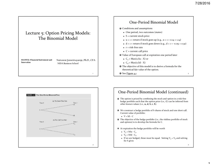
The objective of this model is to derive a formula for the theoretical fair value of the option. See Figure 4.1

3 4

One-Period Binomial Model (continued)

The option is priced by combining the stock and option in a risk-free hedge portfolio such that the option price (i.e., C) can be inferred from

• ther known values (i.e., u, d, S, r, X).

We construct a hedge portfolio of h shares of stock and one short call. Current value of portfolio:

 V = hS - C

The objective of the hedge portfolio (i.e., the riskless portfolio of stock and options) is to develop the formula for C. At expiration the hedge portfolio will be worth

 Vu = hSu - Cu  Vd = hSd - Cd  If we are hedged, these must be equal. Setting Vu = Vd and solving

for h gives

7/28/2016 2

5

One-Period Binomial Model (continued)

These values are all known so h is easily computed Since the portfolio is riskless, it should earn the risk-free

• rate. Thus

 V(1+r) = Vu (or Vd)

Substituting for V and Vu

 (hS - C)(1+r) = hSu – Cu

Substituting for h,

6

One-Period Binomial Model (continued)

This is the theoretical value of the call as determined by the stock price, exercise price, risk-free rate, and up and down factors. Note how the call price is a weighted average of the two possible call prices the next period, discounted at the risk- free rate. The call’s value if the stock goes up (down) in the next period is weighted by the factor p (1-p).

Thus, the theoretical value of the option is

7

One-Period Binomial Model (continued)

An Illustrative Example: S = 100, X = 100, u = 1.25, d = 0.80, r = 0.07 First find the values of Cu, Cd, h, and p:



Cu = Max(0,100(1.25) - 100) = 25



Cd = Max(0,100(.80) - 100) = 0

 h = (25 - 0)/(125 - 80) = 0.556  p = (1.07 - 0.80)/(1.25 - 0.80) = 0.6  Then insert into the formula for C:

8

State Prices

Another way to price options using a binomial model is to define “state price” Specifically, a state price is a present value of a risk neutral price. Where qu is an ‘up’ state price, qd is a ‘down’ state price, p is a risk neutral probability, and r is a risk-free rate per period.

7/28/2016 3

9

State Prices vs Risk-Neutral Prices

10

Two-Period Binomial Model

 We now let the stock go up/down another period so that it

ends up Su2, Sud or Sd2.

 See Figure 4.3.  The option expires after two periods with three possible

values:

11 12

7/28/2016 4

13

After one period the call will have one period to go before

• expiration. Thus, using a single-period model, it will worth

either of the following two values

Two-Period Binomial Model (continued)

In a single-period world, a call option’s value is a weighted average of the option’s two possible values at the end of the next period.

14

Two-Period Binomial Model (continued)

• The hedge ratios are different in the different states:

The price of the call today can again be calculated as a weighted average

• f the two possible call prices in the next period (even if the call does not

expire at the end of the next period); In summary, the two-period binomial option pricing formula provides the

• ption price as a weighted average of the two possible option prices the

next period, discounted at the risk-free rate. The two future option prices, in turn, are obtained from the one-period binomial model.

15

Two-Period Binomial Model (continued)

An Illustrative Example

 Input: S = 100, X = 100, u = 1.25,

d = 0.80, r = 0.07

 Su2 = 100(1.25)2 = 156.25  Sud = 100(1.25)(0.80) = 100  Sd2 = 100(0.80)2 = 64  The call option prices are as

follows

16

Two-Period Binomial Model (continued)

The two values of the call at the end of the first period are The value of p is the same, (1+r-d) / (u-d), regardless of the number of periods in the model.

7/28/2016 5

17

Two-Period Binomial Model (continued)

Therefore, the value of the call today is

18

Pricing Put Options

Pricing a put with the binomial model is the same procedure as pricing a call, except that the expiration payoffs are computed by using put payoff formula. Consider a European put where S = 100, X = 100, u = 1.25, d = 0.80, r = 0.07 In our example the put prices at expiration are;

19

Pricing Put Options

20

Pricing Put Options

The two values of the put at the end of the first period are Therefore, the value of the put today is

P=(1+0.07-0.80)/(1.25-0.80)

7/28/2016 6

21

Pricing American Options

22

American Calls and Early Exercise

The multi-period binomial model is an excellent opportunity to illustrate how American options can be exercised early.

 Consider the American call where

S = 100, X = 100, u = 1.25, d = 0.80, r = 0.07  (the same as the previous European call)

 Now we must consider the possibility of exercising the call early.

At time 1 the European call values were Cu = 31.54 when the stock is at 125 Cd = 0.0 when the stock is at 80

 When the stock is at 125, the call is in-the-money by $25, but it

is still lower than holding value. So not early exercise it. The value of the American call today is now the same at

23

American Calls and Early Exercise

The binomial model can easily accommodate the early exercise of an American call by simply comparing the computed value (holding value) and intrinsic value (exercise value), and select the greater value.

Exercise or intrinsic value = $25 Exercise or intrinsic value = $0 American Call Path

24

American Puts and Early Exercise

The multi-period binomial model is an excellent opportunity to illustrate how American options can be exercised early.

 Consider the American put where

S = 100, X = 100, u = 1.25, d = 0.80, r = 0.07  (the same as the previous European put)

 Now we must consider the possibility of exercising the put early.

At time 1 the European put values were Pu = 0.00 when the stock is at 125 Pd = 13.46 when the stock is at 80

 When the stock is at 80, the put is in-the-money by $20 so

exercise it early. Replace Pu = 13.46 with Pu = 20. The value of the American put today is higher at

7/28/2016 7

25

American Puts and Early Exercise

The binomial model can easily accommodate the early exercise of an American put by simply replacing the computed value with intrinsic value if the latter is greater.

Exercise or intrinsic value

26

Extending the Binomial Model to n Periods

With n periods to go, the binomial model can be easily

• extended. The basic procedure is the same.

See Figure 4.9 in which we see below the stock prices, the prices of European, and American puts. This illustrates the early exercise possibilities for American puts, which can

• ccur in multiple time periods.

At each step, we must check for early exercise by comparing the value if exercised to the value if not exercised and use the higher value of the two.

27

S = 100, X = 100, u = 1.25, d = 0.80, r = 0.07

Early exercise of American put

28

Extending the Binomial Model to n Periods

With n periods and no dividends, the European call price is given as follows; With n periods and no dividends, the European put price is given as follows;

7/28/2016 8

29

Extending the Binomial Model to n Periods

With 3 periods and no dividends, the European call price is given as follows;

30

How to determine parameters (u, d, and risk-free rates) for n periods and a Fixed Option Life

The risk-free rate is adjusted to (1 + r)T/n-1 The up and down parameters are adjusted to

 where  is the annualized volatility.  T is time to maturity in year of the option  n is the number of periods 31

How to determine parameters (u, d, and risk-free rates) for n periods and a Fixed Option Life

Let us price the DCRB June 125 call with TWO periods. The parameters are as follows; the stock price is 125.94, the

• ption has 35 days remaining, the risk-free rate is 4.56

percent per year, and the (annual) DCRB volatility is 83%. p would be (1.00214 - 0.8338)/(1.1993 - 0.8338) = .4606; 1 - p = .5394.

32

How to determine parameters (u, d, and risk-free rates) for n periods and a Fixed Option Life

The new option prices would be

 Cu

2 = Max(0, 181.14 - 125) = 56.14

 Cud = Max(0, 125.94 - 125) = 0.94  Cd

2 = Max(0, 87.56 - 125) = 0.00

So, the prices of the option at time 1 are The price of the option at time 0 is, therefore,

7/28/2016 9

33

Using the Binomial Model to Price Nonstandard Options

The binomial is extremely useful in pricing nonstandard options. For example, there is a call option that allows for early exercise, but the exercise price varies with the time at which you choose to exercise. Let’s consider a call option where there are three exercise dates. The exercise price for each exercise date is as follows;

 Date 1  exercise price = 100.  Date 2  exercise price = 105.  Date 3  exercise price = 110.

What is the price of the option?

34

Using the Binomial Model to Price Nonstandard Options (Con’t)

Consider the following scenario for XYZ stock and its options. XYZ stock is now priced at 100 baht a share. XYZ stock price volatility is historically estimated to be 66% per year. The risk-free rate is 3 percent per year. A European put option on XYZ expiring in four months has an exercise price

• f 105 baht. However, the parties to the option agree that the maximum

payout of this option is 40 baht. (a) Use a three-period binomial model to find the current value of the European put. (b) If there were no limitation on the payoff, what would be the European

• ption price?

(c) What if the maximum payout of this option were set to be 150 baht, what would be the European option price? (d) Compare your answers in (b) and (c). Are they different? Why or why not?