Important Concepts The Black Scholes Merton (BSM) option pricing - - PowerPoint PPT Presentation

1

LECTURE 3.2: OPTION PRICING MODELS: THE BLACK-SCHOLES-MERTON MODEL

Nattawut Jenwittayaroje, PhD, CFA

NIDA Business School National Institute of Development Administration

01135534: Financial Modelling

2

Important Concepts

• The Black‐Scholes‐Merton (BSM) option pricing model

 Black‐Scholes‐Merton Model as the Limit of the Binomial

Model

 Origins of the Black‐Scholes‐Merton Formula  A Nobel Formula

• How to adjust the model to accommodate dividends
• The concepts of historical and implied volatility

 Estimating the Volatility

• BSM option pricing model for put options.

3

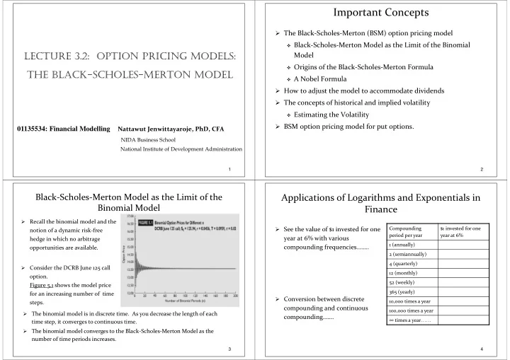
Black‐Scholes‐Merton Model as the Limit of the Binomial Model

• Recall the binomial model and the

notion of a dynamic risk‐free hedge in which no arbitrage

• pportunities are available.
• Consider the DCRB June 125 call
• ption.

Figure 5.1 shows the model price for an increasing number of time steps.

• The binomial model is in discrete time. As you decrease the length of each

time step, it converges to continuous time.

• The binomial model converges to the Black‐Scholes‐Merton Model as the

number of time periods increases.

4

Applications of Logarithms and Exponentials in Finance

• See the value of $1 invested for one

year at 6% with various compounding frequencies……..

• Conversion between discrete

compounding and continuous compounding…….

Compounding period per year $1 invested for one year at 6% 1 (annually) 2 (semiannually) 4 (quarterly) 12 (monthly) 52 (weekly) 365 (yearly) 10,000 times a year 100,000 times a year ∞ times a year……

5

Origins of the Black‐Scholes‐Merton Formula

• Black, Scholes, Merton and the 1997 Nobel Prize

 F. Black and M. S. Scholes. “The Pricing of Options and Corporate

Liabilities.” Journal of Political Economy, 81 (May‐June 1973), 637‐ 659.

 R. C. Merton. “The Theory of Rational Option Pricing.” Bell

Journal of Economics and Management Science, 4 (Spring 1973), 141‐183.

6

A Nobel Formula

• The Black‐Scholes‐Merton model gives the correct formula for a

European call under certain assumptions.

• The general idea of the Black‐Scholes‐Merton model is the same as that
• f the binomial model, except that in BSM model, trading occurs
• continuously. So in BSM, a hedge portfolio is established and maintained

by constantly adjusting the relative proportions of stock and options, a process called dynamic trading.

• The model is derived with complex

mathematics but is easily understandable.

• The Black‐Scholes‐Merton formula

7

A Nobel Formula (continued)

where

 N(d1), N(d2) = cumulative normal

probability

 σ = annualized standard deviation

(volatility) of the continuously compounded (log) return on the stock

 rc = continuously compounded risk-

free rate

 S0= current stock price  X = exercise price  T = time to expiration in years

8

A Digression on Using the Normal Distribution

• The familiar normal, bell‐shaped curve (Figure 5.5)
• See Table 5.1 for determining the normal probability for d1 and
• d2. This gives you N(d1) and N(d2).

9

The cumulative probabilities of the standard normal distribution

10

A Nobel Formula (continued)

• A Numerical Example

 Price the DCRB June 125 call  S0 = 125.94, X = 125, rc = ln(1.0456) = 0.0446, where 4.56% is simple risk‐free

rate, and 4.46% is continuously compounded risk‐free rate

 T = 0.0959,  = 0.83.

11

Black‐Scholes‐Merton Model When the Stock Pays Dividends

• Known Discrete Dividends

 Assume a single dividend of Dt where the ex‐dividend date is time t during

the option’s life.

 Subtract present value of dividends from stock price.  Adjusted stock price, S , is inserted into the B‐S‐M model.  See Table 5.3 for example.

• Continuous Dividend Yield

 Assume the stock pays dividends continuously at the rate of .  Subtract present value of dividends from stock price. Adjusted stock price,

S , is inserted into the B‐S model.

 See Table 5.4 for example.  This approach could also be used if the underlying is a foreign currency,

where the yield is replaced by the continuously compounded foreign risk‐free rate.

12

Black-Scholes-Merton Model When the Stock Pays Discrete Discrete Dividends

13

Black-Scholes-Merton Model When the Stock Pays Contin Continuous uous Dividends

14

Put Option Pricing Models

• Restate put‐call parity with continuous discounting
• Substituting the B‐S‐M formula for C above gives the B‐S‐M put option pricing

model

• The put option can also be represented as;

where N(d1) and N(d2) are the same as in the call model.

• Note calculation of put price:

15

Estimating the Volatility

• There are two approaches to estimating volatility: 1) the historical

volatility, and 2) the implied volatility.

• Historical Volatility

 The historical volatility estimate is based on the assumption that the volatility

that prevailed over the recent past will continue to hold in the future.

 The historical volatility is estimated from a sample of recent continuously

compounded returns on the stock. This is the volatility over a recent time period.

 Collect daily (weekly, or monthly) returns on the stock.  Convert each return to its continuously compounded equivalent by taking ln(1

+ return). Calculate variance.

 Annualize by multiplying by 250 (daily returns), 52 (weekly returns) or 12

(monthly returns). Take square root.

 See Table 5.6 for example with DCRB.

16

Estimating the Historical Volatility

17

Estimating the Implied Volatility

• Implied Volatility

 This is the volatility

implied when the market price of the option is set to the model price.

 Figure 5.17 illustrates the

procedure.

 Substitute estimates of

the volatility into the B‐ S‐M formula until the market price converges to the model price.

18

Interpreting the Implied Volatility

• The CBOE has constructed indices of implied volatility of one‐month at‐the‐

money options based on the S&P 500 (VIX) and Nasdaq (VXN). See Figure 5.20.

• A number of studies have examined whether implied volatility is a good

predictor of the future volatility of a stock. A general consensus is that implied volatility is a better reflection of the appropriate volatility for pricing an

• ption than is the historical volatility.

19

Interpreting the Implied Volatility

VIX is usually referred to as the fear index. It represents

• ne measure of the market’s

expectation of stock market (annualized) volatility over the next 30 day period. For example, if VIX is 20%, the S&P500 is expected to move up or down about 20/sqrt(12) = 5.8% over the next 30 day period. Or there is a 68% likelihood (one SD) that the magnitude of the S&P500’s 30-day return will be less than 5.8% (either up or down).

Source: www.bloomberg.com

S&P500 from Sep 2007 to May 2011 VIX from Sep 2007 to May 2011

20

Summary

• Figure 5.21 shows the relationship between call, put, underlying

asset, risk‐free bond, put‐call parity, and Black‐Scholes‐Merton call and put option pricing models.