Lecture 3.1: Option Pricing The one and two period binomial option - - PowerPoint PPT Presentation

1

Lecture 3.1: Option Pricing Models: The Binomial Model

Nattawut Jenwittayaroje, PhD, CFA

NIDA Business School

National Institute of Development Administration

01135534: Financial Modelling

2

Important Concepts

The concept of an option pricing model The one‐ and two‐period binomial option pricing models Explanation of the establishment and maintenance of a risk‐free hedge Illustration of how early exercise can be captured The extension of the binomial model to any number of time periods

3

One‐Period Binomial Model

Conditions and assumptions

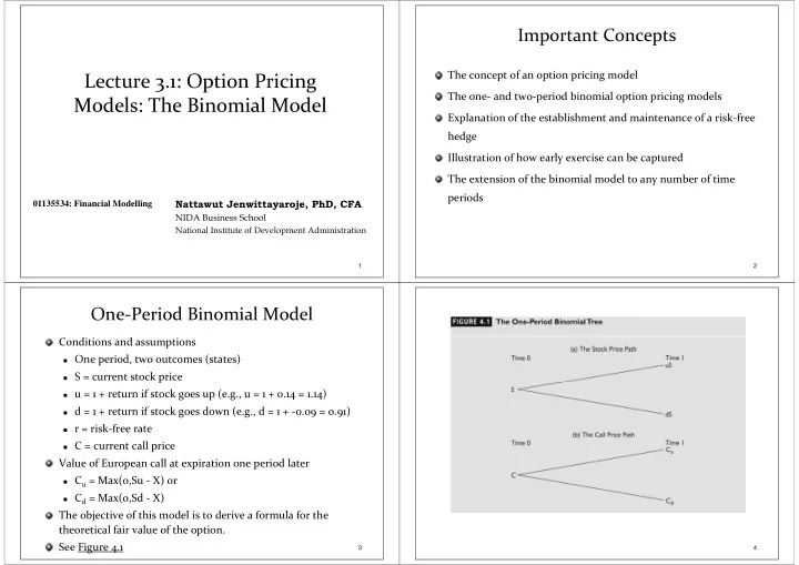
 One period, two outcomes (states)  S = current stock price  u = 1 + return if stock goes up (e.g., u = 1 + 0.14 = 1.14)  d = 1 + return if stock goes down (e.g., d = 1 + ‐0.09 = 0.91)  r = risk‐free rate  C = current call price

Value of European call at expiration one period later

 Cu = Max(0,Su ‐ X) or  Cd = Max(0,Sd ‐ X)

The objective of this model is to derive a formula for the theoretical fair value of the option. See Figure 4.1

4

5

One‐Period Binomial Model (continued)

The option is priced by combining the stock and option in a risk‐free hedge portfolio such that the option price (i.e., C) can be inferred from

• ther known values (i.e., u, d, S, r, X).

We construct a hedge portfolio of h shares of stock and one short call. Current value of portfolio:

 V = hS ‐ C

The objective of the hedge portfolio (i.e., the riskless portfolio of stock and options) is to develop the formula for C. At expiration the hedge portfolio will be worth

 Vu = hSu – Cu , where Cu = Max(0, uS – X)  Vd = hSd ‐ Cd , where Cd = Max(0, dS – X)  If we are hedged, these must be equal. Setting Vu = Vd and solving

for h gives

6

One‐Period Binomial Model (continued)

These values are all known so h is easily computed Since the portfolio is riskless, it should earn the risk‐free

• rate. Thus

 V(1+r) = Vu (or Vd)

Substituting for V and Vu

 (hS ‐ C)(1+r) = hSu – Cu

Substituting for h,

7

One‐Period Binomial Model (continued)

This is the theoretical value of the call as determined by the stock price, exercise price, risk‐free rate, and up and down factors. Note how the call price is a weighted average of the two possible call prices the next period, discounted at the risk‐free rate. The call’s value if the stock goes up (down) in the next period is weighted by the factor p (1‐p). The probabilities of the up and down moves were never specified. They are irrelevant to the option price.

Thus, the theoretical value of the option is

8

One‐Period Binomial Model (continued)

An Illustrative Example

S = 100, X = 100, u = 1.25, d = 0.80, r = 0.07 First find the values of Cu, Cd, h, and p:



Cu = Max(0,100(1.25) ‐ 100) = 25



Cd = Max(0,100(.80) ‐ 100) = 0

 h = (25 ‐ 0)/(125 ‐ 80) = 0.556  p = (1.07 ‐ 0.80)/(1.25 ‐ 0.80) = 0.6  Then insert into the formula for C:

9

One‐Period Binomial Model (continued)

A Hedged Portfolio

 Short 1,000 calls and long 1000h = 1000(0.556) = 556 shares.

See Figure 4.2.

 Value of investment: V = 556($100) ‐ 1,000($14.02)

$41,580. (This is how much money you must put up.)

 Stock goes up to $125

Value of investment = 556($125) ‐ 1,000($25) = $44,500

 Stock goes down to $80

Value of investment = 556($80) ‐ 1,000($0) = $44,480

 You invested $41,580 and got back $44,500, a 7 % return,

which is the risk‐free rate.

10 11

One‐Period Binomial Model (continued)

An Overpriced Call

 Let the call be selling for $15.00  Your amount invested is 556($100) ‐ 1,000($15.00)

= $40,600

 You will still end up with $44,500, which is a 9.6%

return.

 Everyone will take advantage of this, forcing the call

price to fall to $14.02

12

An Underpriced Call

 Let the call be priced at $13  Sell short 556 shares at $100 and buy 1,000 calls at $13.

This will generate a cash inflow of $42,600.

 At expiration, you will end up paying out $44,500.  This is like a loan in which you borrowed $42,600 and

paid back $44,500, a rate of 4.46%, which beats the risk‐free borrowing rate.

One-Period Binomial Model (continued)

13

Two‐Period Binomial Model

 We now let the stock go up/down another period so that it

ends up Su2, Sud or Sd2.

 See Figure 4.3.  The option expires after two periods with three possible

values:

14 15 16

After one period the call will have one period to go before

• expiration. Thus, using a single‐period model, it will worth

either of the following two values

Two‐Period Binomial Model (continued)

In a single‐period world, a call option’s value is a weighted average of the option’s two possible values at the end of the next period.

17

Two‐Period Binomial Model (continued)

• The hedge ratios are different in the different states:

The price of the call today can again be calculated as a weighted average

• f the two possible call prices in the next period (even if the call does not

expire at the end of the next period); In summary, the two‐period binomial option pricing formula provides the

• ption price as a weighted average of the two possible option prices the

next period, discounted at the risk‐free rate. The two future option prices, in turn, are obtained from the one‐period binomial model.

18

Two‐Period Binomial Model (continued)

An Illustrative Example

 Input: S = 100, X = 100, u = 1.25,

d = 0.80, r = 0.07

 Su2 = 100(1.25)2 = 156.25  Sud = 100(1.25)(0.80) = 100  Sd2 = 100(0.80)2 = 64  The call option prices are as

follows

19

Two‐Period Binomial Model (continued)

The two values of the call at the end of the first period are The value of p is the same, (1+r‐d) / (u‐d), regardless of the number of periods in the model.

20

Two‐Period Binomial Model (continued)

Therefore, the value of the call today is

21

Extensions of the Binomial Model

American Calls and Early Exercise Pricing Put Options American Puts and Early Exercise Dividends, European Calls, American Calls, and Early Exercise Extending the Binomial Model to n Periods The Behavior of the Binomial Model for Large n and a Fixed Option Life

22

American Calls and Early Exercise

The multi‐period binomial model is an excellent opportunity to illustrate how American options can be exercised early.

 Consider the American call where

S = 100, X = 100, u = 1.25, d = 0.80, r = 0.07  (the same as the previous European call)

 Now we must consider the possibility of exercising the call early.

At time 1 the European call values were Cu = 31.54 when the stock is at 125 Cd = 0.0 when the stock is at 80

 When the stock is at 125, the call is in‐the‐money by $25, but it

is still lower than holding value. So not early exercise it. The value of the American call today is now the same at

23

American Calls and Early Exercise

The binomial model can easily accommodate the early exercise of an American call by simply comparing the computed value (holding value) and intrinsic value (exercise value), and select the greater value.

Exercise or intrinsic value = $25 Exercise or intrinsic value = $0 American Call Path American Call Path

24

Pricing Put Options

Pricing a put with the binomial model is the same procedure as pricing a call, except that the expiration payoffs are computed by using put payoff formula. Consider a European put where S = 100, X = 100, u = 1.25, d = 0.80, r = 0.07 In our example the put prices at expiration are;

25

Pricing Put Options

26

Pricing Put Options

The two values of the put at the end of the first period are Therefore, the value of the put today is

P=(1+0.07-0.80)/(1.25-0.80)

27

American Puts and Early Exercise

The multi‐period binomial model is an excellent opportunity to illustrate how American options can be exercised early.

 Consider the American put where

S = 100, X = 100, u = 1.25, d = 0.80, r = 0.07  (the same as the previous European put)

 Now we must consider the possibility of exercising the put early.

At time 1 the European put values were Pu = 0.00 when the stock is at 125 Pd = 13.46 when the stock is at 80

 When the stock is at 80, the put is in‐the‐money by $20 so

exercise it early. Replace Pu = 13.46 with Pu = 20. The value of the American put today is higher at

28

American Puts and Early Exercise

The binomial model can easily accommodate the early exercise of an American put by simply comparing the computed value (holding value) and intrinsic value (exercise value), and select the greater value.

Exercise or intrinsic value

29

Dividends, European Calls, American Calls, and Early Exercise

One way to incorporate dividends is to assume a constant yield, , per period. The stock moves up, then drops by the rate . See Figure 4.5, p. 109 for example with a 10% yield The call prices at expiration are The European call prices after one period are The European call value at time 0 is

30

Dividends, European Calls, American Calls, and Early Exercise

If the call is American, when the stock is at 125, it pays a dividend of $12.50 and then falls to $112.50. We can exercise it, paying $100, and receive a stock worth $125. The stock goes ex‐dividend, falling to $112.50 but we get the $12.50

• dividend. So at that point, the option is worth $25. We

replace the binomial value of Cu = $22.78 with Cu = $25. At time 0 the value of the American call is

31

Stock price path with 10% dividend yield at Time 1

The effect of dividend on the early exercise decision

• f an American call, and

hence its value

32

Extending the Binomial Model to n Periods

With n periods to go, the binomial model can be easily

• extended. The basic procedure is the same.

See Figure 4.9, p. 114 in which we see below the stock prices, the prices of European, and American puts. This illustrates the early exercise possibilities for American puts, which can

• ccur in multiple time periods.

At each step, we must check for early exercise by comparing the value if exercised to the value if not exercised and use the higher value of the two.

33

S = 100, X = 100, u = 1.25, d = 0.80, r = 0.07

Early exercise of American put

34

The Behavior of the Binomial Model for Large n and a Fixed Option Life

The risk‐free rate is adjusted to (1 + r)T/n‐1 The up and down parameters are adjusted to

 where  is the annualized volatility. 35

The Behavior of the Binomial Model for Large n and a Fixed Option Life

Let us price the DCRB June 125 call with one period. The parameters are as follows; the stock price is 125.94, the

• ption has 35 days remaining, the risk‐free rate is 4.56

percent per year, and the (annual) DCRB volatility is 83%. The new stock prices are

 Su = 125.9375(1.293087) = 162.8481  Sd = 125.9375(0.773343) = 97.3929 36

The Behavior of the Binomial Model for Large n and a Fixed Option Life

The new option prices would be

 Cu = Max(0,162.8481‐125) = 37.85  Cd = Max(0,97.3929 ‐ 125) = 0.0

p would be (1.004285 ‐ 0.773343)/(1.293087 ‐ 0.773343) = .444; 1 ‐ p = .556. The price of the option at time 0 is, therefore,

37

How to determine parameters (u, d, and risk‐free rates) for n periods and a Fixed Option Life

Let us price the DCRB June 125 call with TWO periods. The parameters are as follows; the stock price is 125.94, the

• ption has 35 days remaining, the risk‐free rate is 4.56

percent per year, and the (annual) DCRB volatility is 83%. p would be (1.00214 ‐ 0.8338)/(1.1993 ‐ 0.8338) = .4606; 1 ‐ p = .5394.

38

How to determine parameters (u, d, and risk‐free rates) for n periods and a Fixed Option Life

The new option prices would be

 Cu

2 = Max(0, 181.14 ‐ 125) = 56.14

 Cud = Max(0, 125.94 ‐ 125) = 0.94  Cd

2 = Max(0, 87.56 ‐ 125) = 0.00

So, the prices of the option at time 1 are The price of the option at time 0 is, therefore,

39

• If we make n large enough, we obtain

a very accurate depiction of what happens to the stock over the option’s life.

• Therefore, we can be confident that
• ur estimated option value is a quite

accurate reflection of the true value of the option.

40

Summary

An option is priced by combining the stock and option in a risk‐ free hedge portfolio such that the option price can be inferred from other known values. The one‐period binomial option pricing formula provides the

• ption price as a weighted average of the two possible option

prices at expiration, discounted at the risk‐free rate. The two‐period binomial option pricing formula provides the

• ption price as a weighted average of the two possible option

prices the next period, discounted at the risk‐free rate, where the two future option prices are obtained from the one‐period binomial model.

41

Summary

Pricing a put with the binomial model is the same procedure as pricing a call, except that the expiration payoffs reflect the put payoff. The binomial model can easily accommodate the early exercise

• f an American option by simply replacing the computed value

with the intrinsic value if the latter is greater. The binomial model converges to a specific value of the option as the number of time periods increases.