Lecture 13: Graphs I: Breadth First Search Lecture Overview - PDF document

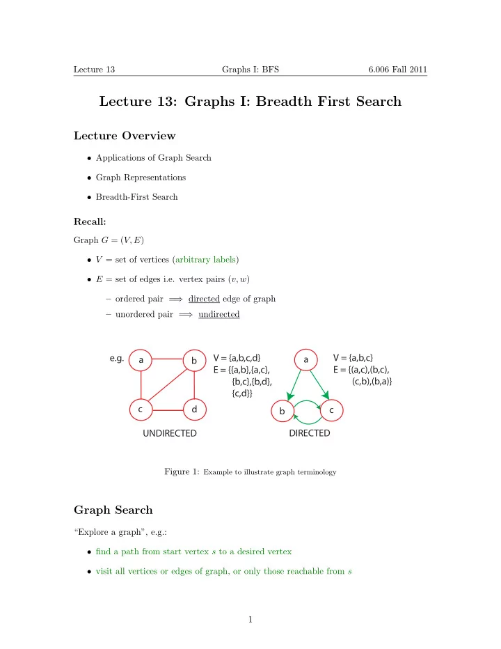
Lecture 13 Graphs I: BFS 6.006 Fall 2011 Lecture 13: Graphs I: Breadth First Search Lecture Overview • Applications of Graph Search • Graph Representations • Breadth-First Search Recall: Graph G = ( V, E ) • V = set of vertices (arbitrary labels) • E = set of edges i.e. vertex pairs ( v, w ) – ordered pair = ⇒ directed edge of graph – unordered pair = ⇒ undirected V = {a,b,c} e.g. V = {a,b,c,d} a a b E = {{a,b},{a,c}, E = {(a,c),(b,c), (c,b),(b,a)} {b,c},{b,d}, {c,d}} c d c b DIRECTED UNDIRECTED Figure 1: Example to illustrate graph terminology Graph Search “Explore a graph”, e.g.: • find a path from start vertex s to a desired vertex • visit all vertices or edges of graph, or only those reachable from s 1

Lecture 13 Graphs I: BFS 6.006 Fall 2011 Applications: There are many. • web crawling (how Google finds pages) • social networking (Facebook friend finder) • network broadcast routing • garbage collection • model checking (finite state machine) • checking mathematical conjectures • solving puzzles and games Pocket Cube: Consider a 2 × 2 × 2 Rubik’s cube Configuration Graph: • vertex for each possible state • edge for each basic move (e.g., 90 degree turn) from one state to another • undirected: moves are reversible Diameter (“God’s Number”) 11 for 2 × 2 × 2, 20 for 3 × 3 × 3, Θ( n 2 / lg n ) for n × n × n [Demaine, Demaine, Eisenstat Lubiw Winslow 2011] “hardest configs” . . . “breadth- solved first tree” possible first moves reachable in two steps but not one 2

Lecture 13 Graphs I: BFS 6.006 Fall 2011 # vertices = 8! · 3 8 = 264 , 539 , 520 where 8! comes from having 8 cubelets in arbitrary positions and 3 8 comes as each cubelet has 3 possible twists. This can be divided by 24 if we remove cube symmetries and further divided by 3 to account for actually reachable configurations (there are 3 connected components). Graph Representations: (data structures) Adjacency lists: Array Adj of | V | linked lists • for each vertex u ∈ V, Adj [ u ] stores u ’s neighbors, i.e., { v ∈ V | ( u, v ) ∈ E } . ( u, v ) are just outgoing edges if directed. (See Fig. 2 for an example.) a c a c a b c b c b Adj Figure 2: Adjacency List Representation: Space Θ( V + E ) • in Python: Adj = dictionary of list/set values; vertex = any hashable object (e.g., int, tuple) • advantage: multiple graphs on same vertices Implicit Graphs: Adj( u ) is a function — compute local structure on the fly (e.g., Rubik’s Cube). This requires “Zero” Space. 3

Lecture 13 Graphs I: BFS 6.006 Fall 2011 Object-oriented Variations: • object for each vertex u • u .neighbors = list of neighbors i.e. Adj [ u ] In other words, this is method for implicit graphs Incidence Lists: • can also make edges objects e.a e e.b • u .edges = list of (outgoing) edges from u . • advantage: store edge data without hashing Breadth-First Search Explore graph level by level from s • level 0 = { s } • level i = vertices reachable by path of i edges but not fewer . . . s level0 last level1 level level2 Figure 3: Illustrating Breadth-First Search 4

Lecture 13 Graphs I: BFS 6.006 Fall 2011 • build level i > 0 from level i − 1 by trying all outgoing edges, but ignoring vertices from previous levels Breadth-First-Search Algorithm BFS (V,Adj,s): See CLRS for queue-based implementation level = { s: 0 } parent = { s : None } i = 1 frontier = [ s ] # previous level, i − 1 while frontier: next = [ ] # next level, i for u in frontier: for v in Adj [ u ] : if v not in level: # not yet seen level [ v ] = i ♯ = level [ u ] + 1 parent [ v ] = u next.append ( v ) frontier = next i + =1 Example level 0 level 1 frontier 0 = {s} 1 0 2 3 frontier 1 = {a, x} a s d f frontier 2 = {z, d, c} frontier 3 = {f, v} 2 2 3 1 z x c v (not x, c, d) level 3 level 2 Figure 4: Breadth-First Search Frontier Analysis: • vertex V enters next (& then frontier) only once (because level[ v ] then set) base case: v = s 5

Lecture 13 Graphs I: BFS 6.006 Fall 2011 • = ⇒ Adj[ v ] looped through only once � | | E for directed graphs � time = | Adj [ V ] | = 2 | E | for undirected graphs v ∈ V • = ⇒ O ( E ) time • O ( V + E ) (“LINEAR TIME”) to also list vertices unreachable from v (those still not assigned level) Shortest Paths: cf. L15-18 • for every vertex v , fewest edges to get from s to v is � level[ v ] if v assigned level ∞ else (no path) • parent pointers form shortest-path tree = union of such a shortest path for each v = ⇒ to find shortest path, take v , parent[ v ], parent[parent[ v ]], etc., until s (or None) 6

MIT OpenCourseWare http://ocw.mit.edu 6.006 Introduction to Algorithms Fall 2011 For information about citing these materials or our Terms of Use, visit: http://ocw.mit.edu/terms.

Lecture 14 Graphs II: DFS 6.006 Fall 2011 Lecture 14: Graphs II: Depth-First Search Lecture Overview • Depth-First Search • Edge Classification • Cycle Testing • Topological Sort Recall: • graph search: explore a graph e.g., find a path from start vertex s to a desired vertex • adjacency lists: array Adj of | V | linked lists – for each vertex u ∈ V , Adj[ u ] stores u ’s neighbors, i.e., { v ∈ V | ( u, v ) ∈ E } (just outgoing edges if directed) For example: a c a c a b c b c b Adj Figure 1: Adjacency Lists Breadth-first Search (BFS): Explore level-by-level from s — find shortest paths 1

Lecture 14 Graphs II: DFS 6.006 Fall 2011 Depth-First Search (DFS) This is like exploring a maze. s Figure 2: Depth-First Search Frontier Depth First Search Algorithm • follow path until you get stuck • backtrack along breadcrumbs until reach unexplored neighbor • recursively explore • careful not to repeat a vertex } } parent = {s: None} search from start vertex s DFS-visit (V, Adj, s): (only see for v in Adj [s]: start stuff reachable v if v not in parent: from s) parent [v] = s finish DFS-visit (V, Adj, v) v DFS (V, Adj) explore parent = { } entire graph for s in V: if s not in parent: (could do same parent [s] = None to extend BFS) DFS-visit (V, Adj, s) Figure 3: Depth-First Search Algorithm 2

Lecture 14 Graphs II: DFS 6.006 Fall 2011 Example cross edge S 1 S 2 1 a b c forward 8 5 edge 2 6 4 f back d e 7 edge 3 back edge Figure 4: Depth-First Traversal Edge Classification tree edges (formed by parent) nontree edges back edge: to ancestor forward edge: to descendant cross edge (to another subtree) Figure 5: Edge Classification • to compute this classification (back or not), mark nodes for duration they are “on the stack” • only tree and back edges in undirected graph Analysis • DFS-visit gets called with a vertex s only once (because then parent[ s ] set) � = ⇒ time in DFS-visit = | Adj[ s ] | = O ( E ) s ∈ V • DFS outer loop adds just O ( V ) = ⇒ O ( V + E ) time (linear time) 3

Lecture 14 Graphs II: DFS 6.006 Fall 2011 Cycle Detection Graph G has a cycle ⇔ DFS has a back edge Proof (<=) tree edges is a cycle back edge: to tree ancestor consider first visit to cycle: (=>) v 3 v 2 v k v 1 v 0 FIRST! • before visit to v i finishes, will visit v i +1 (& finish): will consider edge ( v i , v i +1 ) = ⇒ visit v i +1 now or already did • = ⇒ before visit to v 0 finishes, will visit v k (& didn’t before) • = ⇒ before visit to v k (or v 0 ) finishes, will see ( v k , v 0 ) as back edge Job scheduling Given Directed Acylic Graph (DAG), where vertices represent tasks & edges represent dependencies, order tasks without violating dependencies 4

Lecture 14 Graphs II: DFS 6.006 Fall 2011 8 7 9 G I H 4 2 3 1 C F B A D E 6 5 Figure 6: Dependence Graph: DFS Finishing Times Source: Source = vertex with no incoming edges = schedulable at beginning (A,G,I) Attempt: BFS from each source: • from A finds A, BH, C, F • from D finds D, BE, CF ← slow . . . and wrong! • from G finds G, H • from I finds I Topological Sort  DFS-Visit( v )      . . .   Reverse of DFS finishing times (time at which DFS-Visit( v ) finishes)  order.append( v )     order.reverse()     5

Lecture 14 Graphs II: DFS 6.006 Fall 2011 Correctness For any edge ( u, v ) — u ordered before v , i.e., v finished before u u v • if u visited before v : – before visit to u finishes, will visit v (via ( u, v ) or otherwise) – = ⇒ v finishes before u • if v visited before u : – graph is acyclic – = ⇒ u cannot be reached from v – = ⇒ visit to v finishes before visiting u 6

MIT OpenCourseWare http://ocw.mit.edu 6.006 Introduction to Algorithms Fall 2011 For information about citing these materials or our Terms of Use, visit: http://ocw.mit.edu/terms.