
SLIDE 1
1
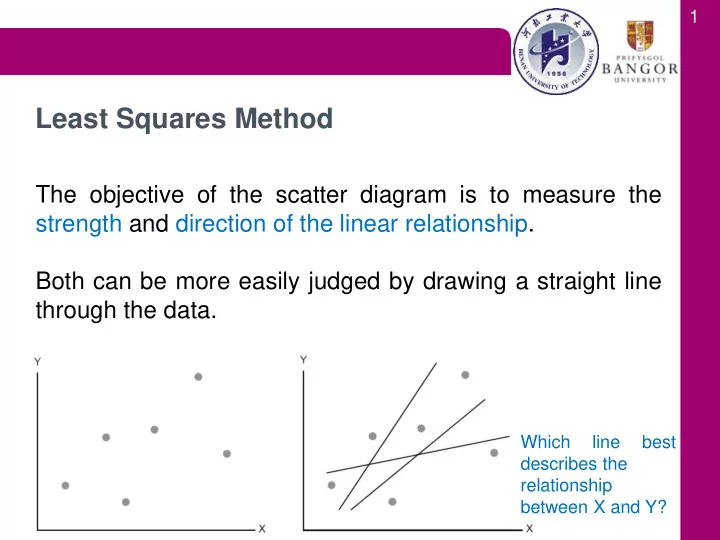
The objective of the scatter diagram is to measure the strength and direction of the linear relationship. Both can be more easily judged by drawing a straight line through the data.
Least Squares Method
Which line best describes the relationship between X and Y?