dixon s random squares method
play

Dixons random squares method Last time we discuss Dixons random - PowerPoint PPT Presentation

Dixons random squares method Last time we discuss Dixons random squares method to factorize a large integer N . The core is to find random squares a 1 , ..., a m such that a 2 i r i (mod N ) such that r i are k -smooth for some small k


  1. Dixon’s random squares method 
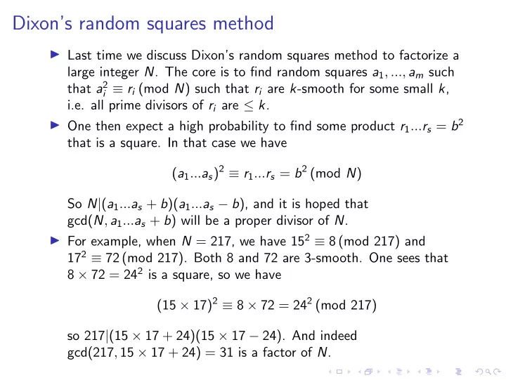
◮ Last time we discuss Dixon’s random squares method to factorize a large integer N . The core is to find random squares a 1 , ..., a m such that a 2 i ≡ r i (mod N ) such that r i are k -smooth for some small k , i.e. all prime divisors of r i are ≤ k . ◮ One then expect a high probability to find some product r 1 ... r s = b 2 that is a square. In that case we have ( a 1 ... a s ) 2 ≡ r 1 ... r s = b 2 (mod N ) So N | ( a 1 ... a s + b )( a 1 ... a s − b ), and it is hoped that gcd( N , a 1 ... a s + b ) will be a proper divisor of N . ◮ For example, when N = 217, we have 15 2 ≡ 8 (mod 217) and 17 2 ≡ 72 (mod 217). Both 8 and 72 are 3-smooth. One sees that 8 × 72 = 24 2 is a square, so we have (15 × 17) 2 ≡ 8 × 72 = 24 2 (mod 217) so 217 | (15 × 17 + 24)(15 × 17 − 24). And indeed gcd(217 , 15 × 17 + 24) = 31 is a factor of N .

  2. Products to be squares ◮ Now comes the question: suppose we have a bunch of r 1 , r 2 , ... r m that are all k -smooth, i.e. having only prime factors among p 1 , ..., p n ≤ k . We can write p e 11 1 p e 12 2 ... p e 1 n r 1 = n p e 21 1 p e 22 2 ... p e 2 n r 2 = n ... p e m 1 1 p e m 2 2 ... p e mn r m = n ◮ Alright, so how do we find a product of the subset of them to be a square? ◮ One easily see that it depends on the quantities e ij for 1 ≤ i ≤ m , 1 ≤ j ≤ n . ◮ The key observation, nevertheless, is that this depends only on the parity of e ij , i.e. e ij mod 2!

  3. Products to be squares, II p e 11 1 p e 12 2 ... p e 1 n r 1 = n p e 21 1 p e 22 2 ... p e 2 n r 2 = n ... p e m 1 1 p e m 2 2 ... p e mn = r m n ◮ Suppose we want to check if a subset S of r 1 , ..., r m has product being a square. Let us define a function f S : { 1 , 2 , ..., m } → { 0 , 1 } to be given by f S ( i ) = 1 if r i is chosen (i.e. r i ∈ S ) and f S ( i ) = 0 if r i �∈ S . ◮ Then what is the product of all r i ∈ S ? It can be expressed as f S ( i )   m m n m n n m n � m r f S ( i ) p e ij p e ij f S ( i ) p e ij f S ( i ) i =1 e ij f S ( i ) � � � � � � � � = = = = p   i j j j j i =1 i =1 j =1 i =1 j =1 j =1 i =1 j =1 ◮ When is such a product a square? Well something like 2 a 3 b 5 c is a square iff all a , b , c are even. Likewise, the above is a square if m � e ij f S ( i ) is even, for every j = 1 , 2 , ..., n . i =1

  4. Linear algebra ◮ So our situation is: given integers e ij ∈ Z ≥ 0 , we want to find f S ( i ) - let’s just abbreviate it as f i - which can be 0 or 1, such that m � e ij f i ≡ 0 (mod 2), for every j = 1 , 2 , ..., n . i =1 ◮ In other words, the problem becomes to find solutions to a system of linear congruence equations mod 2, with constants e ij and variables f i . ◮ The condition that f i ∈ { 0 , 1 } is no longer a problem at all, since mod 2 we only have two elements, represented by 0 and 1, anyway. ◮ So how do we solve system of linear congruence equations? ◮ High school situation: � 3 f + 2 g = 7 6 f + 5 g = 16

  5. Linear algebra mod 2 � 3 f + 2 g = 7 6 f + 5 g = 16 ◮ We typically subtract a multiple of an equation from another so that some variable is killed (in the difference). For example, it looks tempting to subtract from second equation twice of the first. ◮ In other words, we look at the coefficients for a : they are 3 and 6. We subtract 6 / 3 times the first equation to cancel the a -part of the second. ◮ How do we do this mod 2? In fact, we can do the same mod p , because F p is a field! We can divide things like in the rational or real numbers. And thus all those procedures of solving linear systems works the same mod p . ◮ When p = 2, it’s even better cause ... division in F 2 is extremely simple. The only possible divisor - the non-zero element - is 1, and dividing by it does nothing.

  6. Linear algebra mod 2, II ◮ Let us look at an example, suppose we have r 1 = 30, r 2 = 60, r 3 = 10 and r 4 = 24. We rewrite 2 1 · 3 1 · 5 1 r 1 = 2 2 · 3 1 · 5 1 r 2 = 2 1 · 3 0 · 5 1 r 3 = 2 3 · 3 1 · 5 0 r 4 = ◮ To find r f 1 1 ... r f 4 4 to be a square, that is to solve f 1 + 2 f 2 + f 3 + 3 f 4 ≡ 0 (mod 2) f 1 + f 2 + f 4 ≡ 0 (mod 2) f 1 + f 2 + f 3 ≡ 0 (mod 2) ◮ For those of you familiar with matrices, we are looking at transpose     1 1 1 f 1     1 2 1 3 1 2 1 3 2 1 1 f 2  , solving     = 1 1 0 1 1 1 0 1  ≡ 0 (mod 2)        1 0 1 f 3    1 1 1 0 1 1 1 0 3 1 0 f 4

  7. Linear algebra mod 2, III f 1 + 2 f 2 + f 3 + 3 f 4 0 (mod 2) ≡ f 1 + f 2 + f 4 0 (mod 2) ≡ f 1 + f 2 + f 3 0 (mod 2) ≡ ◮ Working mod 2, we can rewrite it mod 2 as f 1 + f 3 + f 4 ≡ 0 (mod 2) f 1 + f 2 + f 4 ≡ 0 (mod 2) f 1 + f 2 + f 3 ≡ 0 (mod 2) ◮ Now suppose we want to cancel the coefficients for f 1 , we can subtract the first equation from the second and third. Noting that 1 − 1 = 0 and 0 − 1 ≡ 1 (mod 2), we have f 1 + f 3 + f 4 ≡ 0 (mod 2) + f 2 + f 3 ≡ 0 (mod 2) + f 2 + f 4 ≡ 0 (mod 2) ◮ Analogously subtract second from the third we havee + + ≡ 0 (mod 2) f 1 f 3 f 4 + + ≡ 0 (mod 2) f 2 f 3 + + ≡ 0 (mod 2) f 3 f 4

  8. Linear algebra mod 2, IV f 1 + f 3 + f 4 0 (mod 2) ≡ + f 2 + f 3 0 (mod 2) ≡ + f 3 + f 4 0 (mod 2) ≡ ◮ Now we can plug in values: say f 4 = 1. Then f 3 ≡ 1 by the third equation. And then f 2 ≡ 1 by the second equation, and finally f 1 ≡ 0 by the first. ◮ Hence for our original r 1 = 30, r 2 = 60, r 3 = 10 and r 4 = 24, we conclude that the product of the last three - excluding r 1 - is a square. ◮ Indeed, 60 × 10 × 24 = 2 6 · 3 2 · 5 2 is a square. ◮ In the scenario above, the leading variables in each equation - f 1 , f 2 and f 3 - are called pivot variables. ◮ They are such that the pivot variable does not appear in latter equations. ◮ The rest non-pivot variables can be arbitrarily assigned values, after which each equation will impose a unique value for its pivot variable, therefore solving the equation. ◮ The same works over any field, in particular F p , just that you need to compute things like 6 / 3 when canceling equations.

Download Presentation
Download Policy: The content available on the website is offered to you 'AS IS' for your personal information and use only. It cannot be commercialized, licensed, or distributed on other websites without prior consent from the author. To download a presentation, simply click this link. If you encounter any difficulties during the download process, it's possible that the publisher has removed the file from their server.

Recommend


More recommend