Learning to Shoot a Goal How do we acquire skill at shooting goals? - - PDF document

SLIDE 1

1

Lecture 8: Learning Models and Skills

CS 344R/393R: Robotics Benjamin Kuipers

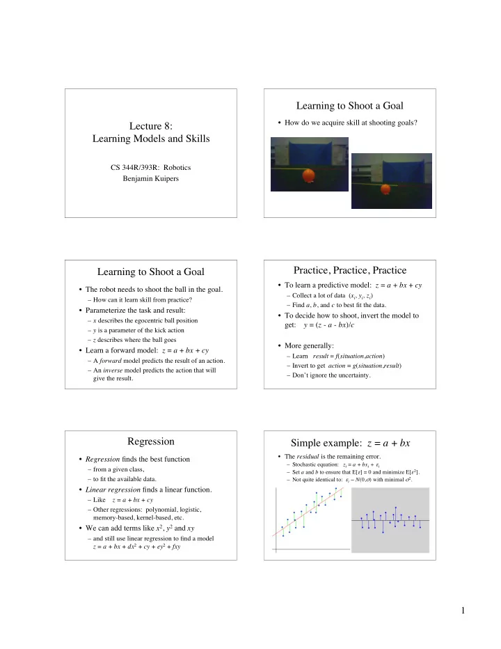
Learning to Shoot a Goal

• How do we acquire skill at shooting goals?

Learning to Shoot a Goal

• The robot needs to shoot the ball in the goal.

– How can it learn skill from practice?

• Parameterize the task and result:

– x describes the egocentric ball position – y is a parameter of the kick action – z describes where the ball goes

• Learn a forward model: z = a + bx + cy

– A forward model predicts the result of an action. – An inverse model predicts the action that will give the result.

Practice, Practice, Practice

• To learn a predictive model: z = a + bx + cy

– Collect a lot of data (xi, yi, zi) – Find a, b, and c to best fit the data.

• To decide how to shoot, invert the model to

get: y = (z - a - bx)/c

• More generally:

– Learn result = f(situation,action) – Invert to get action = g(situation,result) – Don’t ignore the uncertainty.

Regression

• Regression finds the best function

– from a given class, – to fit the available data.

• Linear regression finds a linear function.

– Like z = a + bx + cy – Other regressions: polynomial, logistic, memory-based, kernel-based, etc.

• We can add terms like x2, y2 and xy

– and still use linear regression to find a model z = a + bx + dx2 + cy + ey2 + fxy

Simple example: z = a + bx

• The residual is the remaining error.

– Stochastic equation: zi = a + bxi + εi – Set a and b to ensure that E[ε] = 0 and minimize E[ε2]. – Not quite identical to: εi ∼ N(0,σ) with minimal σ2.

SLIDE 2

2

First, the simple case …

• Suppose we have n data points (xi, zi)

– and we want to learn a model z = a + bx + ε

• We need to find a and b to minimize the

squared error:

• Shift the mean to the origin:
• First we find b such that

– Once we have b, we will get E = (zi

i=1 n

• a bxi)2

(xi x , zi z ) (zi z ) = b(xi x ) a = z bx

After shifting the data to the origin

• Given the data set

– look for the best fit b for – that minimizes

• Look for a local minimum of E
• It’s a minimum because

(xi x , zi z ) (z z ) = b(x x ) E = (zi

i=1 n

• z b(xi x

))2

dE db = 2(zi z b(xi x )) (xi x )

1 n

• =

= 2 (zi z )(xi x ) b(xi x )2

( )

1 n

• =

b = (zi z )(xi x )

• (xi x

)2

• d2E

db2 = +2 (xi x )2

• > 0

Summary

• Given n data points (xi, zi)

– The best fitting line z = a + bx is given by

b = (zi z )(xi x )

• (xi x

)2

• a = z bx

Up to more dimensions …

• Suppose our dataset is (xi, yi, zi)

– (For simplicity, assume data centered at origin) – We want to fit the plane z = bx + cy

• The error term is
• Find a minimum
• Solve for b and c

E = (zi

i=1 n

• bxi cyi)2

E b = 2xi(zi bxi cyi)

• = 0

E c = 2yi(zi bxi cyi)

• = 0

b xi

2

• +

c xiyi

• =

xizi

• b

xiyi

• +

c yi

2

• =

yizi

• Caution!
• It’s easy to listen to this, and even read it

carefully, and think it all makes sense.

– But you still don’t understand it!

• Your dataset (xi, yi, zi) will not be centered

around the origin.

– You need to fit the plane z = a + bx + cy

• Work through the math for this, by hand.

Cleaning the data

• Given the data (xi, yi, zi)

– find the best-fitting plane z = a + bx + cy

• Compute the residuals: ri = zi − a − bxi − cyi

– The mean of the ri should be zero. – Compute the standard deviation σr

• A data point is an outlier if |ri| > 3σr

– Discard the outliers

• Recompute the regression, using only inliers.

SLIDE 3

3

Discarding Outliers

• Why is it OK to discard outliers if |ri| > 3σr ?

– Outliers are still data, aren’t they?

• A model explains data by saying that some

causes are relevant, and others are negligible.

• If a data point has p < .001 according to the

model, it is more likely explained as a modeling error, than as an unlikely outcome.

– An unlikely outcome isn’t helpful in fitting model parameters, anyway.

Hough Transform

• Representing a line

x cos θ + y sin θ = r (x,y)⋅(cos θ, sin θ) = r

For fixed (r,θ), represent all points (x,y) on a given line. For fixed (x,y), represent all lines (r,θ) through (x,y).

Hough Space: (r,θ) representations

• Each observed point (x,y) votes for all lines (r,θ)

passing through it.

Votes From Three Points

• Each point contributes a curve of votes.

Lines Get the Most Votes

• Votes from three very strong lines.

Lines Get the Most Votes

• Identify local max in Hough Space to define

a line in Image Space.

SLIDE 4

4

Hough Transform Issues

• Hough Transform works with any

parameterized model: circle, rectangle, etc.

– But in a high-dimensional Hough Space, each cell gets few votes

• To maximize votes, use large cells.

– But they give low resolution model descriptions.

RANSAC Random Sample Consensus

• A method for robust model-fitting.

– Separating inliers from outliers.

RANSAC to Find Line Models

• Repeat k times:

– Select 2 points from data, to define a model M. – Collect all points from data, within tolerance t

• f the model M. These are the inliers.
• If #inliers < d, give up on model M.

– Find the model M′ that best fits the inliers.

• In this case, by linear regression.

– Record the error of the inliers from model M′.

• Return the model M′ with the lowest error.

RANSAC Pros and Cons

• Very robust search for models.

– The model classifies data as inliers and outliers

• Can estimate probability of failure as a

function of k. But no upper bound.

• Can find multiple models by deleting data

explained by current best model.

– But this can fail if current best model is bad.

Back to Learning a Skill!

• Remember:

– x describes the egocentric ball position – y is a parameter of the kick action – z describes where the ball goes

• Learn a forward model: z = a + bx + cy

– Practice to collect the data (xi, yi, zi) – Do regression to find a, b, and c

• To decide how to shoot, invert the model to

get: y = (z - a - bx)/c

Learning to Shoot a Goal

Ball position x. Goal position z. Kick param y

SLIDE 5

5

Egocentric Ball Position: x

• I assume that you can position your robot so

that the ball position can be described by a single parameter x.

– You can use (x1, x2), but more variables requires more data.

• When you’re close enough to kick the ball,

you’ll be too close to be sure where it is!

– Pick a position farther away, for accurate x.

Kick Action parameter: y

• The built-in kicks have no parameters.
• Your kick action includes a step or two to

approach the ball, then a built-in kick.

– Embed the parameter y in the approach.

• Try various parameterizations:

– Sideways component of the walk – Turning while walking forward – etc.

• Avoid gaps in the search space of y values.

Where the ball goes: z

• Track the ball after the kick.

– “Keep your eye on the ball!”

• After a suitable period of time (1 second?),

record the direction the ball went.

– Body-centered egocentric frame of reference

Planning the shot

• You have a forward model: z = a + bx + cy
• Invert the model: y = (z - a - bx)/c

– z is where you want the ball to go – x is where you see the ball right now – a, b, c have been learned – Compute y: how to control the kick action

• Q: Would it help to have a Bayesian model
• f the distribution p(z | x, y)?

Next

• Kalman filters: tracking dynamic systems.
• Extended Kalman filters: handling

nonlinearity by local linearization.