Lattice Points and Kindly Chess Queens Thomas Zaslavsky Binghamton - - PDF document

CombinaTexas 10: 26 April 2009

Lattice Points and Kindly Chess Queens

Thomas Zaslavsky Binghamton University of SUNY

Jointly with Matthias Beck, Seth Chaiken, and Christopher R.H. Hanusa

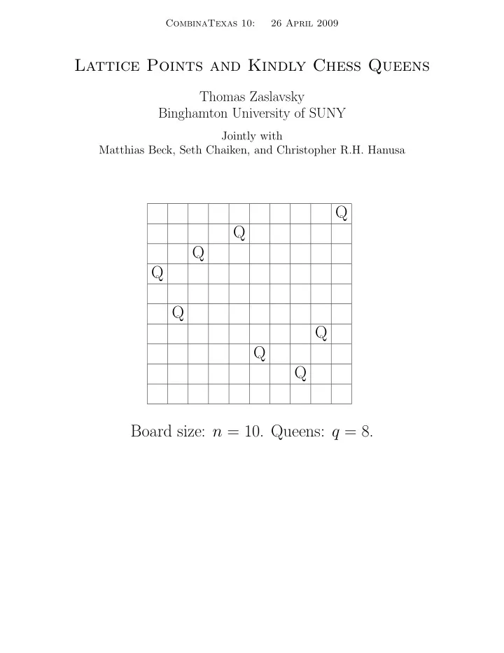
Q Q Q Q Q Q Q Q Board size: n = 10. Queens: q = 8.

An n × n board: q identical chess pieces: P P P · · · P P Put the pieces on the board! The pieces are kindly and do not wish to attack each other. The Question: How many ways are there to do this, as a function of n? NP(q; n) NQ(n; n) ? (The n-queens problem.)

Coordinate system: y x Pi Pj Pi coordinates: (xi, yi) ∈ Z2 ⊆ R2. Configuration: (x1, y1, . . . , xq, yq) ∈ R2q. Moves: αµk where µk = (µk1, µk2) ∈ MP and α ∈ Z. Attack: (xj, yj) − (xi, yi) ∈ µk. Permitted configurations: (x1, y1, . . . , xq, yq) ∈ {1, 2, . . . , n}2q = (0, n + 1)2q ∩ Z2q. Forbidden hyperplanes: Hk,i,j : [(xj, yj) − (xi, yi)] · µ⊥

k = 0, in R2q.

The count: NP(q; n) = # of integer points in (n + 1)(0, 1)2q \

• k,i,j

Hk,i,j.

Polytopes and Ehrhart theory Convex polytope P in Rδ with rational vertices. EP(t) := # of integer points in tP, for t = 1, 2, . . . . d := least common denominator of all vertices. Theorem 1 (Ehrhart, Macdonald). (a) EP(t) is a quasipolynomial function of t > 0 with leading term vol(P)tδ. (b) Its period p divides d. (c) EP◦(t) = (−1)δEP(−t). (Ehrhart reciprocity.) Quasipolynomial f(t): It is p polynomials f1(t), . . . , fp(t) with f(t) := ft mod p(t). Its period is p. Example: P = [0, 1]δ, vol(P) = 1, p = 1. (Integral vertices give a polynomial.) Computation: LattE computes the number of points for fixed t.

Inside-out polytopes Convex polytope P with rational vertices. Finite set of rational hyperplanes H of hyperplanes, all in Rδ. EP,H(t) := # of integer points in tP but not in

• H.

Theorem 2 (Beck & Zaslavsky). The Ehrhart properties (a–c) hold for EP,H(t). Also: (d) (−1)δE◦

P◦,H(0) is the number of regions of P as dissected by H.

Reduction to standard Ehrhart theory via L := the set of non-empty intersections of hyperplanes in P◦,

• rdered by reverse inclusion so 0 = P◦, and

µ(0, u) = M¨

• bius function of L.

Theorem 3 (Beck & Zaslavsky). E◦

P◦,H(t) =

• u∈L

µ(0, u)EP◦∩u(t). Example: P = [0, 1]δ, vol(P) = 1, period p ≫ 1 with forbidden hyperplanes.

Chromatic polynomials via Ehrhart Graphs. χΓ(λ) := number of proper colorations of Γ with colors 1, 2, . . . , λ = E◦

P◦,H(λ + 1)

(i.e., t = λ + 1), where P = [0, 1]|V | and H = {xi = xj : ∃ eij}. Integral vertices. Denominator: 1. Period: 1. Conclusion: One monic polynomial of degree |V |. Signed graphs. Σ := graph with + and − edges. χΣ(2k + 1) := number of proper colorations of Σ with colors 0, ±1, ±2, . . . , ±k = E◦

P◦,H(2k + 2)

(i.e., t = 2k + 2), χ∗

Σ(2k) := number of proper colorations of Σ with colors ± 1, ±2, . . . , ±k

= E◦

P◦,H(2k + 1)

(i.e., t = 2k + 1), where P = [0, 1]|V | and H = (1

2, . . . , 1 2) + {xi = sgn(eij)xj : ∃ eij}.

Half-integral vertices. Denominator: 2. Period: 1 or 2. Conclusion: Two monic polynomials of degree |V |.

The count of non-attacking configurations With a chess piece P: δ = 2q, P = [0, 1]2q. H = {Hk,i,j : 1 ≤ k ≤ # of basic moves, 1 ≤ i < j ≤ q}, NP(n) = E◦

P◦,H(n + 1)

(i.e., t = n + 1). NP(−1) = E◦

P◦,H(0) = the number of combinatorial types of configuration.

The hyperplanes are given by a matrix: MP :=   µ⊥

1

µ⊥

2

. . .   ,

• ne line for each basic move, and D(Kn).

Period p? (Needed for computer calculation.) Hard! A bound p′ for p = ⇒ the quasipolynomial by computer calculation of all polynomial constituents of all EP◦∩u(t) in Theorem 3 using LattE. ∴ Task: To bound p for every q. An upper bound is d. ∴ Task: To bound d for every q. Hard!

The period For the chess problem we need: lcmd(A) := least common multiple of all subdeterminants of A. Kronecker product: A ⊗ B := a11B a12B . . . . . . . . . ...

• .

Proposition 4 (Hanusa & Zaslavsky). Let A be a 2 × 2 matrix, not identically zero, and q ≥ 1. The least common multiple of all square minor determinants of A ⊗ D(Kq) is lcmd

• A ⊗ D(Kq)
• = lcm
• (lcmd A)q−1,

⌊q/2⌋

LCM

p=2

• (a11a22)p − (a12a21)p⌊q/2p⌋

. For a chess piece, B = D(Kq). For the bishop or queen, A =

• 1

1 1 −1

• r
• 1 0 1

1 1 0 1 −1

• from (MP)T.

Apply Proposition 4, using lcmd(A) = 2. We get lcmd

• A ⊗ D(Kq)
• = 2q−1,

an upper bound on d, hence on the period p, for q bishops or queens.

The bishop MB =

• 1

1 1 −1

• ,

lcmd(MB) = 2. For two bishops, NB(2; n) = n(n − 1)(3n2 − n + 2) 6 = n 6

• 3n3 − 4n2 + 3n − 2
• .

For 3 and more bishops we haven’t yet done the computer work. The queen MQ =     1 1 1 1 1 −1     , lcmd(MQ) = 2. For two queens, NQ(2; n) = n(n − 1)(3n2 − 7n + 2) 6 = n 6

• 3n3 − 10n2 + 9n − 2
• .

For 3 or more queens we’ll need computer work.

Reading Assignment Ehrhart theory. * Matthias Beck and Sinai Robins, Computing the Continuous Discretely: Integer-Point Enumeration in Polyhedra. Undergraduate Texts in Mathematics. Springer, New York, 2007. Matthias Beck and Thomas Zaslavsky, Inside-out polytopes. Advances in Math. 205 (2006), no. 1, 134–162. Other. Seth Chaiken, Christopher R.H. Hanusa, and Thomas Zaslavsky, A q-queens problem. (In preparation.) Christopher R.H. Hanusa and Thomas Zaslavsky, Determinants in the Kronecker product of matrices: The incidence matrix of a complete

• graph. (In preparation.)