Last Time: Summary. Hypercube Eigenvalues of hypercube. V = { 0 , 1 - - PowerPoint PPT Presentation

SLIDE 1

Last Time: Summary.

Graph G = (V,E), assume regular graph of degree d. Edge Expansion. h(S) =

|E(S,V−S)| d min|S|,|V−S|, h(G) = minS h(S)

M = A/d adjacency matrix, A Eigenvector: a vector v where Mv = λv Spectral theorem: Eigenvectors form basis: v1,...,vn. x = α1v1 +α2v2 +···αnvn. Mx = α1λ1v1 +α2λ2v2 +···αnλnvn Highest eigenvalue: λ1 = 1. Proof: Plug in 1. Second Eigenvalue: λ2 < 1 if connected. Proof: v2 is not v1. Eigenvalue gap: µ = λ1 −λ2. Cheeger: µ

2 ≤ h(G) ≤ =

• 2µ

Proof of LHI: Plug in “cut” vector,x, into Rayleigh Quotient. µ = 1−maxx⊥1 xtMx

xtx .

This expression ’counts’ edges in cut ’x’ plus scales by volume. Yields h(S).

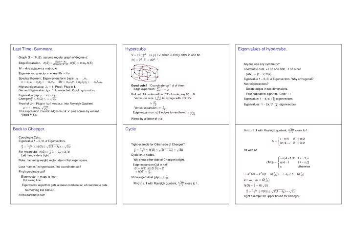
Hypercube

V = {0,1}d (x,y) ∈ E when x and y differ in one bit. |V| = 2d |E| = d2d−1. Good cuts? “Coordinate cut”: d of them. Edge expansion:

2d−1 d2d−1 = 1 d

Ball cut: All nodes within d/2 of node, say 00···0. Vertex cut size: d

d/2

• bit strings with d/2 1’s.

≈ 2d

√ d

Vertex expansion: ≈

1 √ d .

Edge expansion: d/2 edges to next level. ≈

1 2 √ d

Worse by a factor of √ d

Eigenvalues of hypercube.

Anyone see any symmetry? Coordinate cuts. +1 on one side, -1 on other. (Mv)i = (1−2/d)vi. Eigenvalue 1−2/d. d Eigenvectors. Why orthogonal? Next eigenvectors? Delete edges in two dimensions. Four subcubes: bipartite. Color ±1 Eigenvalue: 1−4/d. d

2

• eigenvectors.

Eigenvalues: 1−2k/d. d

k

• eigenvectors.

Back to Cheeger.

Coordinate Cuts: Eigenvalue 1−2/d. d Eigenvectors.

µ 2 = 1−λ2 2

≤ h(G) ≤

• 2(1−λ2) =
• 2µ

For hypercube: h(G) = 1

d λ1 −λ2 = 2/d.

Left hand side is tight. Note: hamming weight vector also in first eigenspace. Lose “names” in hypercube, find coordinate cut? Find coordinate cut? Eigenvector v maps to line. Cut along line. Eigenvector algorithm gets a linear combination of coordinate cuts. Something like ball cut. Find coordinate cut?

Cycle

Tight example for Other side of Cheeger?

µ 2 = 1−λ2 2

≤ h(G) ≤

• 2(1−λ2) =
• 2µ

Cycle on n nodes. Will show other side of Cheeger is tight. Edge expansion:Cut in half. |S| = n/2, |E(S,S)| = 2 → h(G) = 2

n.

Show eigenvalue gap µ ≤ 1

n2 .

Find x ⊥ 1 with Rayleigh quotient, xT Mx

xT x close to 1.

Find x ⊥ 1 with Rayleigh quotient, xT Mx

xT x close to 1.

xi =

• i −n/4

if i ≤ n/2 3n/4−i if i > n/2 Hit with M. (Mx)i =      −n/4+1/2 if i = 1,n n/4−1 if i = n/2 xi

• therwise

→ xT Mx = xT x(1−O( 1

n2 ))

→ λ2 ≥ 1−O( 1

n2 )

µ = λ1 −λ2 = O( 1

n2 )

h(G) = 2

n = Θ(√µ) µ 2 = 1−λ2 2

≤ h(G) ≤

• 2(1−λ2) =
• 2µ

Tight example for upper bound for Cheeger.

SLIDE 2

Eigenvalues of cycle?

Eigenvalues: cos 2πk

n .

xi = cos 2πki

n

(Mx)i = cos

• 2πk(i+1)

n

• +cos
• 2πk(i−1)

n

• = 2cos
• 2πk

n

• cos
• 2πki

n

• Eigenvalue: cos 2πk

n .

Eigenvalues: vibration modes of system. Fourier basis.

Random Walk.

p - probability distribution. Probability distrubtion after choose a random neighbor. Mp. Converge to uniform distribution. Power method: Mtx goes to highest eigenvector. Mtx = a1λ t

1v1 +a2λ2v2 +···

λ1 −λ2 - rate of convergence. Ω(n2) steps to get close to uniform. Start at node 0, probability distribution, [1,0,0,··· ,0]. Takes Ω(n2) to get n steps away. Recall drunken sailor. Eigenvalues, random walks, volume estimation, counting.

Sampling.

Sampling: Random element of subset S ⊂ {0,1}n or {0,...,k}k. Related Problem: Approximate |S| within factor of 1+ε. Random walk to do both for some interesting sets S.

Convex Bodies.

S ⊂ [k]n is grid points inside Convex Body. Ex: Numerically integrate convex function in d dimensions. Compute ∑i viVol(f(x) > vi) where vi = iδ. Example: P defined by set of linear inequalities. Or other “membership oracle” for P S is set of grid points inside Convex Body. Grid points that satisfy linear inequalities.

• r “other” membership oracle.

Choose a uniformly random elt? Easy to choose randomly from [k]n which is big. For convex body? Choose random point in [k]n and check if in P. Works. But P could be exponentially small compared to |[k]n|. Takes a long time to even find a point in P.

Convex Body Graph.

S ⊂ [k]n is set of grid points inside Convex Body. Sample Space: S. Graph on grid points inside P or on Sample Space. One neighbor in each direction for each dimension (if neighbor is inside P.) Degree: 2d. How big is graph? Big! So big it ..it INSERT JOKE HERE. O(kn) if coordinates in [k]. That’s a big graph! How to find a random node? Start at a grid point, and take a (random) walk. When close to uniform distribution...have a sample point. How long does this take? More later. But remember power method...which finds first eigenvector.

SLIDE 3

Spanning Trees.

Problem: How many? Another Problem: find a random one. Algorithm: Start with spanning tree. Repeat: Swap a random nontree edge with a random tree edge. How long? Sample space graph (BIG GRAPH) of spanning trees. Node for each tree. Neighboring trees differ in two edges. Algorithm is random walk on BIG GRAPH (sample space graph.)

Spin systems.

Each element of S may have associated weight. Sample element proportional to weight. Example? 2 or 3 dimensional grid of particles. Particle State ±1. System State {−1,+1}n. Energy on local interactions: E = ∑(i,j) −σiσj. “Ferromagnetic regime”: same spin is good. Gibbs distribution ∝ e−E/kT . Physical properties from Gibbs distribution. Metropolis Algorithm: At x, generate y with a single random flip. Go to y with probability min(1,w(y)/w(x)) Random walk in sample space graph (BIG GRAPH ALERT) (not random walk in 2d grid of particles.) Markov Chain on statespace of system.

Sampling structures and the BIG GRAPH

Sampling Algorithms ≡ Random walk on BIG GRAPH. Small degree.

Vertices Neighbors Degree (ish) Grid points in convex body. Change one dimension 2d Spanning Trees. Change two edges. ≤ |V|2 neighbors per node Spin States. Change one spin O(n) neighbors.

Analyzing random walks on graph.

Start at vertex, go to random neighbor. For d-regular graph: eventually uniform. if not bipartite. Odd /even step! How to analyse? Random Walk Matrix: M. M - normalized adjacency matrix. Symmetric, ∑j M[i,j] = 1. M[i,j]- probability of going to j from i. Probability distribution at time t: vt. vt+1 = Mvt Each node is average over neighbors. Evolution? Random walk starts at 1, distribution e1 = [1,0,...,0]. Mtv1 = 1

N v1 +∑i>1 λ t i αivi.

v1 = [ 1

N ,..., 1 N ] →Uniform distribution.

Doh! What if bipartite? Negative eigenvalues of value -1: (+1,−1) on two sides. Side question: Why the same size? Assumed regular graph.

Fix-it-up chappie!

“Lazy” random walk: With probability 1/2 stay at current vertex. Evolution Matrix: I+M

2

Eigenvalues: 1+λi

2 1 2(I +M)vi = 1 2(vi +λivi) = 1+λi 2 vi

Eigenvalues in interval [0,1]. Spectral gap: 1−λ2

2

= µ

2 .

Uniform distribution: π = [ 1

N ,..., 1 N ]

Distance to uniform: d1(vt,π) = ∑i |(vt)i −πi| “Rapidly mixing”: d1(vt,π) ≤ ε in poly(logN,log 1

ε ) time.

When is chain rapidly mixing? Another measure: d2(vt,π) = ∑i((vt)i −πi)2. Note: d1(vt,π) ≤ √ Nd2(vt,π) n – “size” of vertex, µ ≥

1 p(n) for poly p(n), t = O(p(n)logN).

d2(vt,π) = |Ate1 −π|2 ≤

• (1+λ2)

2

2t ≤ (1−

1 2p(n))2t ≤ 1

poly(N) Rapidly mixing with big (≥

1 p(n)) spectral gap.

Rapid mixing, volume, and surface area..

Recall volume of convex body. Grid graph on grid points inside convex body. Recall Cheeger: µ

2 ≤ h(G) ≤

• 2µ.

Lower bound expansion → lower bounds on spectral gap µ → Upper bound mixing time. h(G) ≈ Surface Area Volume Isoperimetric inequality. Voln−1(S,S) ≥ min(Vol(S),Vol(S))

diam(P)

Edges ∝ surface area, Assume Diam(P) ≤ p′(n) → h(G) ≥ 1/p′(n) → µ > 1/2p′(n)2 → O(p′(n)2 logN) convergence for Markov chain on BIG GRAPH. → Rapidly mixing chain:

SLIDE 4

Khachiyan’s algorithm for counting partial orders.

Given partial order on x1,...,xn. Sample from uniform distribution over total orders. Start at an ordering. Swap random pair and go if consistent with partial order. Rapidly mixing chain? Map into d-dimensional unit cube. xi < xj corresponds to halfspace (one side of hyperplane) of cube. “dimension i = dimension j” total order is intersection of n halfspaces. each of volume: 1

n!.

since each total order is disjoint and together cover cube.

(0,0) x1 > x2 x1 > x2 x1 > x3 x2 > x3 (0,0) x1 > x2 x1 > x2 x1 > x3 x2 > x3

Each order takes 1

n! volume.

Number of orders ≡ volume of intersection of partial order relations. Diameter: O(√n) Isoperimetry: Voln−1(S,S) = E(S,S)

(n−1)! ≥ |S| n!√n

Edge Expansion: the degree d is O(n2), h(S) = |E(S,S)|

d|S|

≥

1 n7/2 Mixes in time O(n7 logN) = O(n8 logn).

Do the polynomial dance!!!

Summary.

Eigenvectors for hypercubes. Tight example for LHI of Cheeger. Eigenvectors for cycle. Tight example for RHI of Cheeger. Random Walks and Sampling. Eigenvectors, Isoperimetry of Volume, Mixing. Partial Order Application.