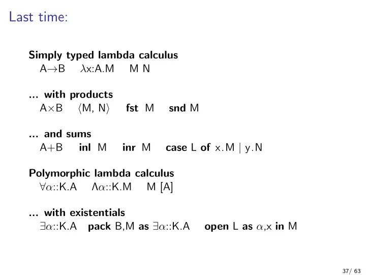
Last time: Simply typed lambda calculus A B x:A.M M N ... with - PowerPoint PPT Presentation

Last time: Simply typed lambda calculus A → B λ x:A.M M N ... with products A × B � M, N � fst M snd M ... and sums A+B inl M inr M case L of x.M | y.N Polymorphic lambda calculus ∀ α ::K.A Λ α ::K.M M [A] ... with existentials ∃ α ::K.A pack B,M as ∃ α ::K.A open L as α ,x in M 37/ 63

Typing rules for existentials Γ ⊢ M : A [ α := B ] Γ ⊢ ∃ α :: K . A :: ∗ ∃ -intro Γ ⊢ pack B , M as ∃ α :: K . A : ∃ α :: K . A Γ ⊢ M : ∃ α :: K . A Γ , α :: K , x : A ⊢ M ′ : B ∃ -elim Γ ⊢ open M as α, x in M ′ : B 38/ 63

Unit in OCaml type u = Unit 39/ 63

Encoding data types in System F: unit The unit type has one inhabitant . We can represent it as the type of the identity function . Unit = ∀ α : : ∗ . α → α The unit value is the single inhabitant: u n i t = Λ α . λ a : α . a We can package the type and value as an existential : pack ( ∀ α : : ∗ . α → α , Λ α . λ a : α . a ) as ∃ U : : ∗ . u We’ll write 1 for the unit type and �� for its inhabitant. 40/ 63

Booleans in OCaml A boolean data type: bool = False | True type A destructor for bool: i f : bool − > ’ a − > ’ a − > ’ a val i f b then e l s e = l e t match b with False − > e l s e | True − > then 41/ 63

Encoding data types in System F: booleans The boolean type has two inhabitants: false and true . We can represent it using sums and unit. Bool = 1+1 The constructors are represented as injections: f a l s e = i n l [ 1 ] �� true = i n r [ 1 ] �� The destructor ( if ) is implemented using case : λ b : Bool . Λ α : : ∗ . λ r : α . λ s : α . case b of x . s | y . r 42/ 63

Encoding data types in System F: booleans We can package the definition of booleans as an existential: pack (1+1 , � i n r [ 1 ] �� , � i n l [ 1 ] �� , λ b : Bool . Λ α : : ∗ . λ r : α . λ s : α . case b of x . s | y . r �� ) as ∃ β : : ∗ . β × β × ( β → ∀ α : : ∗ . α → α . α ) 43/ 63

Natural numbers in OCaml A nat data type type nat = Zero : nat | Succ : nat − > nat A destructor for nat : val foldNat : nat − > ’ a − > ( ’ a − > ’ a ) − > ’ a l e t rec foldNat n z s = match n with Zero − > z | Succ n − > s ( foldNat n z s ) 44/ 63

Encoding data types in System F: natural numbers The type of natural numbers is inhabited by Z , SZ , SSZ , ... We can represent it using a polymorphic function of two parameters: N = ∀ α : : ∗ . α → ( α → α ) → α The Z and S constructors are represented as functions: z : N z = Λ α : : ∗ . λ z : α . λ s : α → α . z s : N → N s = λ n : ∀ α : : ∗ . α → ( α → α ) → α . Λ α : : ∗ . λ z : α . λ s : α → α . s (n [ α ] z s ) , The fold N destructor allows us to analyse natural numbers: f o l d N : N → ∀ α . α → ( α → α ) → α f o l d N = λ n : ∀ α : : ∗ . α → ( α → α ) → α . n 45/ 63

Encoding data types: natural numbers (continued) f o l d N : N → ∀ α . α → ( α → α ) → α For example, we can use fold N to write a function to test for zero: λ n : N . f o l d N n [ Bool ] true ( λ b : Bool . f a l s e ) Or we could instantiate the type parameter with N and write an addition function: λ m: N . λ n : N . f o l d N m [ N ] n succ 46/ 63

Encoding data types: natural numbers (concluded) Of course, we can package the definition of N as an existential: pack ( ∀ α : : ∗ . α → ( α → α ) → α , � Λ α : : ∗ . λ z : α . λ s : α → α . z , � λ n : ∀ α : : ∗ . α → ( α → α ) → α . Λ α : : ∗ . λ z : α . λ s : α → α . s (n [ α ] z s ) , � λ n : ∀ α : : ∗ . α → ( α → α ) → α . n ��� ) as ∃ N :: ∗ . N × ( N → N ) × ( N → ∀ α . α → ( α → α ) → α ) 47/ 63

System F ω (polymorphism + type abstraction) 48/ 63

System F ω by example A kind for binary type operators ∗⇒∗⇒∗ A binary type operator λα : : ∗ λβ : : ∗ . α + β A kind for higher-order type operators ( ∗⇒∗ ) ⇒∗⇒∗ A higher-order type operator λφ : : ∗ ⇒∗ . λα : : ∗ . φ ( φ α ) 49/ 63

Kind rules for System F ω K 1 is a kind K 2 is a kind ⇒ -kind K 1 ⇒ K 2 is a kind 50/ 63

Kinding rules for System F ω Γ ⊢ A :: K 1 ⇒ K 2 Γ , α :: K 1 ⊢ A :: K 2 Γ ⊢ B :: K 1 ⇒ -intro ⇒ -elim Γ ⊢ λα :: K 1 . A :: K 1 ⇒ K 2 Γ ⊢ A B :: K 2 51/ 63

Sums in OCaml ( ’ a , ’b) sum = type I n l : ’ a − > ( ’ a , ’ b) sum | I n r : ’b − > ( ’ a , ’ b) sum val case : ( ’ a , ’b) sum − > ( ’ a − > ’ c ) − > ( ’ b − > ’ c ) − > ’ c l e t case s l r = match s with I n l x − > l x | I n r y − > r y 52/ 63

Encoding data types in System F ω : sums We can finally define sums within the language. As for N sums are represented as a binary polymorphic function: Sum = λα : : ∗ . λβ : : ∗ . ∀ γ : : ∗ . ( α → γ ) → ( β → γ ) → γ The inl and inr constructors are represented as functions: i n l = Λ α : : ∗ . Λ β : : ∗ . λ v : α . Λ γ : : ∗ . λ l : α → γ . λ r : β → γ . l v i n r = Λ α : : ∗ . Λ β : : ∗ . λ v : β . Λ γ : : ∗ . λ l : α → γ . λ r : β → γ . r v The foldSum function behaves like case : foldSum = Λ α : : ∗ . Λ β : : ∗ . λ c : ∀ γ : : ∗ . ( α → γ ) → ( β → γ ) → γ . c 53/ 63

Encoding data types: sums (continued) Of course, we can package the definition of Sum as an existential: pack λα : : ∗ . λβ : : ∗ . ∀ γ : : ∗ . ( α → γ ) → ( β → γ ) → γ , Λ α : : ∗ . Λ β : : ∗ . λ v : α . Λ γ : : ∗ . λ l : α → γ . λ r : β → γ . l v Λ α : : ∗ . Λ β : : ∗ . λ v : β . Λ γ : : ∗ . λ l : α → γ . λ r : β → γ . r v Λ α : : ∗ . Λ β : : ∗ . λ c : ∀ γ : : ∗ . ( α → γ ) → ( β → γ ) → γ . c as ∃ φ : : ∗ ⇒∗⇒∗ . ∀ α : : ∗ . ∀ β : : ∗ . α → φ α β × ∀ α : : ∗ . ∀ β : : ∗ . β → φ α β × ∀ α : : ∗ . ∀ β : : ∗ . φ α β → ∀ γ : : ∗ . ( α → γ ) → ( β → γ ) → γ (However, the pack notation becomes unwieldy as our definitions grow.) 54/ 63

Lists in OCaml A list data type: type ’ a l i s t = N i l : ’ a l i s t | Cons : ’ a ∗ ’ a l i s t − > ’ a l i s t A destructor for lists: val f o l d L i s t : ’ a l i s t − > ’b − > ( ’ a − > ’b − > ’b) − > ’b l e t rec f o l d L i s t l n c = l match with N i l − > n | Cons ( x , xs ) − > c x ( f o l d L i s t xs n c ) 55/ 63

Encoding data types in System F: lists We can define parameterised recursive types such as lists in System F ω . As for N lists are represented as a binary polymorphic function: L i s t = λα : : ∗ . ∀ φ : : ∗ ⇒∗ . φ α → ( α → φ α → φ α ) → φ α The nil and cons constructors are represented as functions: n i l = Λ α : : ∗ . Λ φ : : ∗ ⇒∗ . λ n : φ α . λ c : α → φ α → φ α . n cons = Λ α : : ∗ . λ x : α . λ xs : L i s t α . Λ φ : : ∗ ⇒∗ . λ n : φ α . λ c : α → φ α → φ α . c x ( xs [ φ ] n c ) The destructor corresponds to the foldList function: f o l d L i s t = Λ α : : ∗ . Λ β : : ∗ . λ c : α → β → β . λ n : β . λ l : L i s t α . l [ λγ : : ∗ . β ] n c 56/ 63

Encoding data types: lists (continued) We defined add for N , and we can define append for lists: append = Λ α : : ∗ . λ l : L i s t α . λ r : L i s t α . f o l d L i s t [ α ] [ L i s t α ] l r ( cons [ α ] ) 57/ 63

Nested types in OCaml A regular type: type ’ a t r e e = Empty : ’ a t r e e | Tree : ’ a t r e e ∗ ’ a ∗ ’ a t r e e − > ’ a t r e e A non-regular type: type ’ a p e r f e c t = ZeroP : ’ a − > ’ a p e r f e c t | SuccP : ( ’ a ∗ ’ a ) p e r f e c t − > ’ a p e r f e c t 58/ 63

Encoding data types in System F ω : nested types We can represent non-regular types like perfect in System F ω : P e r f e c t = λα : : ∗ . ∀ φ : : ∗ ⇒∗ . ( ∀ α : : ∗ . α → φ α ) → ( ∀ α : : ∗ . φ ( α × α ) → φ α ) → φ α This time the arguments to zeroP and succP are themselves polymorphic: zeroP = Λ α : : ∗ . λ x : α . Λ φ : : ∗ ⇒∗ . λ z : ∀ α : : ∗ . α → φ α . λ s : φ ( α × α ) → φ α . z [ α ] x succP = Λ α : : ∗ . λ p : P e r f e c t ( α × α ) . Λ φ : : ∗ ⇒∗ . λ z : ∀ α : : ∗ . α → φ α . λ s : ( ∀ β : : ∗ . φ ( β × β ) → φ β ) . s [ α ] (p [ φ ] z s ) 59/ 63

Encoding data types in System F ω : Leibniz equality Recall Leibniz’s equality: consider objects equal if they behave identically in any context In System F ω : Eq = λα : : ∗ . λβ : : ∗ . ∀ φ : : ∗ ⇒∗ . φ α → φ β Equality is reflexive ( A ≡ A ): r e f l = Λ α : : ∗ . Λ φ : : ∗ ⇒∗ . λ x : φ α . x and symmetric ( A ≡ B → B ≡ A ): symm = Λ α : : ∗ . Λ β : : ∗ . λ e : ( ∀ φ : : ∗ ⇒∗ . φ α → φ β ) . e [ λγ : : ∗ . Eq γ α ] ( r e f l [ α ] ) and transitive ( A ≡ B ∧ B ≡ C → A ≡ C ): t r a n s = Λ α : : ∗ . Λ β : : ∗ . Λ γ : : ∗ . λ ab : Eq α β . λ bc : Eq β γ . bc [ Eq α ] ab 60/ 63