[PPT] - Laplace Transforms Laplace Transform Motivation Definition v s ( t PowerPoint Presentation

SLIDE 1

Laplace Transform Motivation Continued Why are we studying the Laplace transform?

– Easier than working with multiple differential equations – More general than the types of analysis we discussed in ECE 221

– Controls (ECE 311) – Communications – Signal Processing – Analog circuits (ECE 32X sequence)

Laplace Transforms

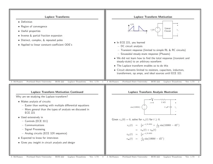
Laplace Transform Analysis Illustration

Given vo(0) = 0, solve for vo(t) for t ≥ 0. vo(t) =

= vtr(t) + vss(t) vtr(t) =

vss(t) =

Laplace Transform Motivation

t Linear Circuit vs(t)

vs(t)

– DC circuit analysis – Transient response (limited to simple RL & RC circuits) – Sinusoidal steady-state response (Phasors)

steady-state) to an arbitrary waveform

transformers, op amps, and ideal sources until ECE 321

SLIDE 2

Approach

analysis will not become apparent for several lectures

Laplace Transform Analysis Illustration Continued

5 10 15 20 25 −0.8 −0.6 −0.4 −0.2 0.2 0.4 0.6 0.8 1 Total Transient Steady State

vo(t) =

= vtr(t) + vss(t)

Laplace Transform Definition L {x(t)} = X(s) ∞

X(s) = +∞

+ Easier to obtain the transient response + Consistent with common practice – Ignores x(t) for t < 0

Laplace Transform for ODE’s

x(t) Linear Circuit

ak dky(t) dtk =

bk dkx(t) dtk

constant-coefficient ordinary differential equation (ODE)

Mechanical, Chemical, Biological, etc.

techniques of differential equations or convolution

SLIDE 3

Example 2: Laplace Transform of x(t) Find the Laplace transform of x(t) = e−atu(t). What is the region of convergence? What is the transform of x(t) = e−at?

Laplace Transform Convergence

signals and all values of s

– Sinusoids – e−atu(t) for any real |a| < ∞ – δ(t)

called the region of convergence (ROC)

classes on linear systems

Example 3: Laplace Transform of x(t) Find the Laplace transform of x(t) = δ(t). What is the region of convergence?

Example 1: Laplace Transform of x(t) Find the Laplace transform of x(t) = u(t). What is the region of convergence? What is the transform of x(t) = 1?

SLIDE 4

Laplace Transform Properties

– Improves our understanding of the transform – Enables us to find the transform more easily – Enables us to find the inverse transform more easily

x(t) u(t)

⇐ ⇒ X(s) X(s) = L {x(t)} x(t) u(t) = L−1 {X(s)}

Example 4: Laplace Transform of x(t) Find the Laplace transform of x(t) = cos(ωt)u(t). What is the region

Linearity X1(s) = L {x1(t)} X2(s) = L {x2(t)} then you should be able to show that [a1x1(t) + a2x2(t)] u(t)

⇐ ⇒ a1X1(s) + a2X2(s) Example: Find the Laplace transform of x(t) = 5δ(t) − 2 cos 5t. L {δ(t)} = 1 L {cos ωt} = s s2 + ω2 L {5δ(t) − 2 cos 5t} = 5(1) − 2

s2 + 52

5 − 2s s2 + 25

Example 4: Workspace

SLIDE 5

Translation in Frequency Given X(s) = L {x(t)}, what is the inverse Laplace transform of X(s + s0)? X(s + s0) = ∞

= ∞

e−st dt = L

= e−s0tx(t) u(t) e−s0tx(t) u(t)

⇐ ⇒ X(s + s0)

Scaling Given X(s) = L {x(t)}, what is L {x(at)} for a > 0? L {x(at)} = ∞

τ = at t = τ a dτ = a dt dt = 1 a dτ L {x(at)} = 1 a ∞

= 1 a ∞

x(at) u(t)

⇐ ⇒ 1 aX s a

Time Differentiation Given X(s) = L {x(t)}, what is the Laplace transform of ˙ x(t)? L dx(t) dt

∞

dx(t) dt e−st dt u = e−st du = −se−st dt dv = dx(t) dt dt v = x(t) L dx(t) dt

∞

∞

= e−stx(t)

∞

dt =

∞

dx(t) dt u(t)

⇐ ⇒ sX(s) − x(0−)

Translation in Time Given X(s) = L {x(t)}, what is L {x(t − t0) u(t − t0)} for t0 > 0? L {x(t − t0)u(t − t0)} = ∞

τ = t − t0 dτ = dt t = τ + t0 L {x(t − t0) u(t − t0)} = ∞

x(τ) u(τ)e−s(τ+t0) dτ = ∞

= e−st0 ∞

x(t − t0) u(t − t0)

⇐ ⇒ e−st0X(s)

SLIDE 6

Other Properties

687)

to the exams

Time Differentiation Continued In general dnx(t) dtn u(t)

⇐ ⇒ snX(s) − sn−1x(0−) − · · · − s0 dn−1x(t) dtn−1

If all of the initial conditions are zero, dnx(t) dt u(t)

⇐ ⇒ snX(s)

Example 5: Laplace Transform Properties Find the Laplace transform of t u(t).

Time Integration Given X(s) = L {x(t)}, what is the Laplace transform of t

L t x(τ) dτ

∞

t x(τ) dτ

u = t x(τ) dτ du = x(t) dt dv = e−stdt v = −1 s e−st L t x(τ) dτ

t x(τ) dτ −1 s e−st

− ∞

−1 s e−stx(t) dt = (0 − 0) + 1 s ∞

t x(τ) dτ

⇐ ⇒ 1 sX(s)

SLIDE 7

Inverse Laplace Transform Overview L−1 {X(s)} = 1 j2π σ1+j∞

X(s) est ds

convergence

Example 6: Laplace Transform Properties Find the Laplace transform of ˙ r(t) dr(t) dt

Inverse Laplace Transform Example X(s) = s + 8 s(s + 2) = 4 s − 3 s + 2 Since we know u(t)

⇐ ⇒ 1 s e−atu(t)

⇐ ⇒ 1 s + a a1x1(t)u(t) + a2x2(t)u(t)

⇐ ⇒ a1X1(s) + a2X2(s) we know that the inverse Laplace transform of X(s) is L−1 {X(s)} = 4u(t) − 3e−2tu(t)

Example 7: Laplace Transform Properties Find the Laplace transform of e−at cos(ωt) u(t). Hint: L {cos(ωt)} =

SLIDE 8

PFE: Distinct Poles X(s) = N(s) D(s) = N(s) (s + p1)(s + p2) . . . (s + pn) = k1 s + p1 + k2 s + p2 + · · · + kn s + pn ki = (s + pi)X(s)|s=−pi

Partial Fraction Expansion A critical step in the previous example was finding following equation: X(s) = s + 8 s(s + 2) = 4 s − 3 s + 2

similar tool

Example 8: Partial Fraction Expansion Given X(s) = L {x(t)}, find x(t). X(s) = 5s + 29 s3 + 8s2 + 19s + 12

PFE: Overview In general, most functions will have a general form X(s) = N(s) D(s) = N

M

SLIDE 9

PFE: Distinct Complex Poles Method 2 X(s) = N(s) D(s) = k1s + k2 s2 + as + b + R(s) = k1s + k1α + k2 − k1α (s + α)2 + β2 + R(s) = k1(s + α) + k2 − k1α (s + α)2 + β2 + R(s) = c1(s + α) (s + α)2 + β2 + c2β (s + α)2 + β2 + R(s) c1 = k1 c2 = k2 − k1α β x(t) = c1e−αt cos(βt)u(t) + c2e−αt sin(βt)u(t) + L−1 {R(s)}

Example 8: Workspace

Example 9: Distinct Complex Poles Given X(s) = L {x(t)}, find x(t) using both methods of handling complex poles. X(s) = 2 s3 + 2s2 + 2s

PFE: Distinct Complex Poles Method 1 X(s) = N(s) D(s) = N(s) (s + α − jβ)(s + α + jβ) = k1 s + α − jβ + k∗

s + α + jβ k1 = (s + α − jβ)X(s)|s=−α+jβ

conjugate pairs

SLIDE 10

PFE: Repeated Poles X(s) = N(s) D(s) = N(s) (s + p)n = k1 s + p + k2 (s + p)2 + · · · + kn (s + p)n kn−m = 1 m! d(m) dsm (s + p)nX(s)|s=−p L−1

(s + p)n

1 (n − 1)!tn−1e−ptu(t)

Example 9: Workspace

Example 10: Repeated Poles Given X(s) = L {x(t)}, find x(t). X(s) = s − 2 s(s + 1)3

PFE: Useful Transforms k s + a ⇔ ke−atu(t) k (s + a)2 ⇔ kte−atu(t) k s + α − jβ + k∗ s + α + jβ ⇔ 2|k|e−αt cos(βt + θk)u(t) k (s + α − jβ)2 + k∗ (s + α + jβ)2 ⇔ 2t|k|e−αt cos(βt + θk)u(t) where k = |k|∠θk

SLIDE 11

Solving Ordinary Differential Equations

ak dky(t) dtk = x(t)

akskY (s) −

sk−ℓy(ℓ−1)(0−) = X(s) Y (s) = X(s) + N

k

N

If L {x(t)} is a rational function of s, then the linear ordinary differential equation shown above can be solved (more easily) using the Laplace Transform

Example 10: Workspace

Example 11: Solving ODE’s Solve the following ODE for y(t) given that y(0−) = ˙ y(0−) = 0 d2y(t) dt2 + 3dy(t) dt + 2y(t) = 20 cos(2t)u(t) + 1

Hint:

PFE: Improper Rational Functions X(s) = N(s) D(s) = A(s) + B(s) C(s)

expression that contains a proper rational function

partial fraction expansion

SLIDE 12

Summary

equations

and the properties of the transform

Example 11: Workspace 1

Example 11: Workspace 2