Laplace Transforms Circuit Analysis Example 1: Circuit Analysis We - - PowerPoint PPT Presentation

laplace transforms circuit analysis example 1 circuit
SMART_READER_LITE
LIVE PREVIEW

Laplace Transforms Circuit Analysis Example 1: Circuit Analysis We - - PowerPoint PPT Presentation

Laplace Transforms Circuit Analysis Example 1: Circuit Analysis We can use the Laplace transform for circuit analysis if we can define Passive element equivalents the circuit behavior in terms of a linear ODE. Review of ECE 221 methods in


slide-1
SLIDE 1

Example 1:Workspace Hint:

≫ [r,p,k] = residue([-2e-3 2e3],[1 1e6 0]) r = -0.0040, 0.0020, p = -1000000, 0 k = []

  • J. McNames

Portland State University ECE 222 Laplace Circuits

  • Ver. 1.63

3

Laplace Transforms Circuit Analysis

  • Passive element equivalents
  • Review of ECE 221 methods in s domain
  • Many examples
  • J. McNames

Portland State University ECE 222 Laplace Circuits

  • Ver. 1.63

1

Example 1:Workspace

  • J. McNames

Portland State University ECE 222 Laplace Circuits

  • Ver. 1.63

4

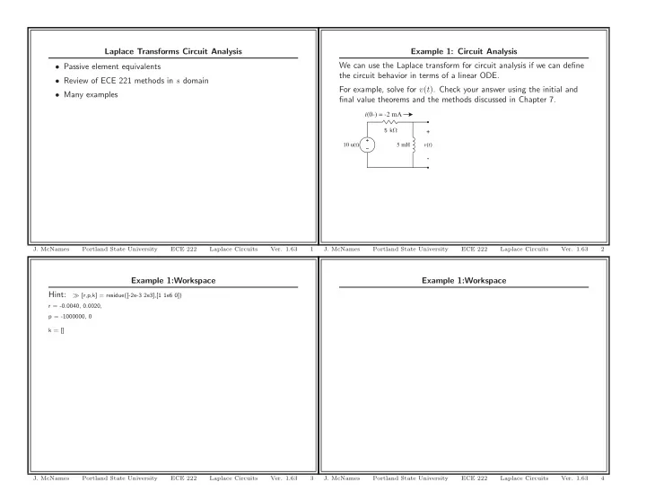
Example 1: Circuit Analysis We can use the Laplace transform for circuit analysis if we can define the circuit behavior in terms of a linear ODE. For example, solve for v(t). Check your answer using the initial and final value theorems and the methods discussed in Chapter 7.

10 u(t) v(t)

  • +

5 mH

i(0-) = -2 mA

5 kΩ

  • J. McNames

Portland State University ECE 222 Laplace Circuits

  • Ver. 1.63

2

slide-2
SLIDE 2

Defining s Domain Equations: Resistors

R v(t)

  • +

i(t) R V(s)

  • +

I(s)

v(t) = R i(t) V (s) = R I(s)

  • Generalization of Ohm’s Law
  • As with KCL & KVL, the relationship is the same in the s domain

as in the time domain

  • Note that we used the linearity property of the LPT for both

Ohm’s law and Kirchhoff’s laws

  • J. McNames

Portland State University ECE 222 Laplace Circuits

  • Ver. 1.63

7

Laplace Transform Circuit Analysis Overview

  • LPT is useful for circuit analysis because it transforms differential

equations into an algebra problem

  • Our approach will be similar to the phasor transform
  • 1. Solve for the initial conditions

– Current flowing through each inductor – Voltage across each capacitor

  • 2. Transform all of the circuit elements to the s domain
  • 3. Solve for the s domain voltages and currents of interest
  • 4. Apply the inverse Laplace transform to find time domain

expressions

  • How do we know this will work?
  • J. McNames

Portland State University ECE 222 Laplace Circuits

  • Ver. 1.63

5

Defining s Domain Equations: Inductors

v(t)

  • +

i(t) L V(s)

  • +

I(s) Ls L I0 V(s)

  • +

I(s) Ls I0 s

v(t) = Ldi(t) dt i(t) = 1 L t

0- v(τ) dτ + I0

V (s) = L [sI(s) − I0] I(s) = 1 sLV (s) + 1 sI0 V (s) = sLI(s) − LI0 Where I0 i(0-)

  • J. McNames

Portland State University ECE 222 Laplace Circuits

  • Ver. 1.63

8

Kirchhoff’s Laws

N

  • k=1

vk(t) = 0

N

  • k=1

Vk(s) = 0

M

  • k=1

ik(t) = 0

M

  • k=1

Ik(s) = 0

  • Kirchhoff’s laws are the foundation of circuit analysis

– KVL: The sum of voltages around a closed path is zero – KCL: The sum of currents entering a node is equal to the sum

  • f currents leaving a node
  • If Kirchhoff’s laws apply in the s domain, we can use the same

techniques that you learned last term (ECE 221)

  • Apply the LPT to both sides of the time domain expression for

these laws

  • The laws hold in the s domain
  • J. McNames

Portland State University ECE 222 Laplace Circuits

  • Ver. 1.63

6

slide-3
SLIDE 3

s Domain Circuit Element Summary Resistor V (s) = RI(s) V = RI

R

Inductor V (s) = sLI(s) V = sLI

Ls

Capacitor V (s) =

1 sC I(s)

V =

1 sC I

1 sC

  • All of these are in the form V (s) = ZI(s)
  • Note similarity to phasor transform
  • Identical if s = jω
  • Will discuss further later
  • Equations only hold for zero initial conditions
  • J. McNames

Portland State University ECE 222 Laplace Circuits

  • Ver. 1.63

11

Defining s Domain Equations: Capacitors

v(t)

  • +

i(t) V(s)

  • +

I(s) V(s)

  • +

I(s) CV0 C 1 sC V0 s 1 sC

i(t) = C dv(t) dt v(t) = 1 C t

0- i(τ) dτ + V0

I(s) = C [sV (s) − V0] V (s) = 1 C 1 sI(s)

  • + 1

sV0 I(s) = sCV (s) − CV0 V (s) = 1 sC I(s) + V0 s Where V0 v(0-)

  • J. McNames

Portland State University ECE 222 Laplace Circuits

  • Ver. 1.63

9

Example 2: Circuit Analysis

10 u(t) v(t)

  • +

5 mH

i(0-) = -2 mA

5 kΩ

Solve for v(t) using s-domain circuit analysis.

  • J. McNames

Portland State University ECE 222 Laplace Circuits

  • Ver. 1.63

12

s Domain Impedance and Admittance Impedance: Z(s) = V (s) I(s) Admittance: Y (s) = I(s) V (s)

  • The s domain impedance of a circuit element is defined for zero

initial conditions

  • This is also true for the s domain admittance
  • We will see that circuit s domain circuit analysis is easier when we

can assume zero initial conditions

  • J. McNames

Portland State University ECE 222 Laplace Circuits

  • Ver. 1.63

10

slide-4
SLIDE 4

Example 3: Workspace Hint:

≫ [r,p,k] = residue([1e6],conv([1 0 1e6],[1 1e3])) r = [ 0.5000, -0.2500 - 0.2500i, -0.2500 + 0.2500i] p = 1.0e+003 *[ -1.0000, 0.0000 + 1.0000i, 0.0000 - 1.0000i] k = [] ≫ [abs(r) angle(r)*180/pi] ans = [ 0.5000 0, 0.3536 -135.0000, 0.3536 135.0000]

  • J. McNames

Portland State University ECE 222 Laplace Circuits

  • Ver. 1.63

15

Example 2: Workspace

  • J. McNames

Portland State University ECE 222 Laplace Circuits

  • Ver. 1.63

13

Example 3: Workspace

  • J. McNames

Portland State University ECE 222 Laplace Circuits

  • Ver. 1.63

16

Example 3: Circuit Analysis

t = 0 vo

  • +

1 kΩ sin(1000t) 1 µF

Given vo(0) = 0, solve for vo(t) for t ≥ 0.

  • J. McNames

Portland State University ECE 222 Laplace Circuits

  • Ver. 1.63

14

slide-5
SLIDE 5

Example 4: Workspace Hint:

≫ [r,p,k] = residue([1e-3 20 0],[1 21.25e3 10e3]) r = [-1.2496, -0.0004] p = [-21250,-0.4706] k = [0.0010]

  • J. McNames

Portland State University ECE 222 Laplace Circuits

  • Ver. 1.63

19

Example 3: Plot of Results

5 10 15 20 25 −0.8 −0.6 −0.4 −0.2 0.2 0.4 0.6 0.8 1 Total Transient Steady State

Time (ms) vo(t) (V)

  • J. McNames

Portland State University ECE 222 Laplace Circuits

  • Ver. 1.63

17

Example 4: Workspace

  • J. McNames

Portland State University ECE 222 Laplace Circuits

  • Ver. 1.63

20

Example 4: Circuit Analysis 40 V 10 mF 10 mH t = 0 v

  • +

50 Ω 50 Ω 100 Ω 175 Ω 175 Ω

Solve for v(t).

  • J. McNames

Portland State University ECE 222 Laplace Circuits

  • Ver. 1.63

18

slide-6
SLIDE 6

Example 6: Workspace Hint:

≫ [r,p,k] = residue([98e3],[1 400 1e6]) r = [ 0 -50.0104i, 0 +50.0104i] p = 1.0e+002 * [ -2.0000 + 9.7980i, -2.0000 - 9.7980i] k = [] ≫ [abs(r) angle(r)*180/pi] ans =[ 50.0104 -90.0000, 50.0104 90.0000]

  • J. McNames

Portland State University ECE 222 Laplace Circuits

  • Ver. 1.63

23

Example 5: Parallel RLC Circuits

C L R v(t)

  • +

i(t)

Find an expression for V (s). Assume zero initial conditions.

  • J. McNames

Portland State University ECE 222 Laplace Circuits

  • Ver. 1.63

21

Example 6: Workspace

  • J. McNames

Portland State University ECE 222 Laplace Circuits

  • Ver. 1.63

24

Example 6: Circuit Analysis

8 H v

  • +

iL

20 kΩ 0.125 µF

Given v(0) = 0 V and the current through the inductor is iL(0-) = −12.25 mA, solve for v(t).

  • J. McNames

Portland State University ECE 222 Laplace Circuits

  • Ver. 1.63

22

slide-7
SLIDE 7

Example 7: Series RLC Circuits

R L C v(t) vR(t)

  • +

vL(t)

  • +

vC(t)

  • +

Find an expression for VR(s), VL(s), and VC(s). Assume zero initial conditions.

  • J. McNames

Portland State University ECE 222 Laplace Circuits

  • Ver. 1.63

27

Example 6: Plot of v(t)

5 10 15 20 25 30 35 40 −40 −20 20 40 60 80 Time (ms) (volts)

  • J. McNames

Portland State University ECE 222 Laplace Circuits

  • Ver. 1.63

25

Example 7: Workspace

  • J. McNames

Portland State University ECE 222 Laplace Circuits

  • Ver. 1.63

28

Example 6: MATLAB Code

t = 0:0.01e-3:40e-3; v = 50*exp(-200*t).*sin(979.8*t); t = t*1000; h = plot(t,v,’b’); set(h,’LineWidth’,1.2); xlim([0 max(t)]); ylim([-23 40]); box off; xlabel(’Time (ms)’); ylabel(’(volts)’); title(’’);

  • J. McNames

Portland State University ECE 222 Laplace Circuits

  • Ver. 1.63

26

slide-8
SLIDE 8

Example 8: Workspace

  • J. McNames

Portland State University ECE 222 Laplace Circuits

  • Ver. 1.63

31

Example 8: Circuit Analysis

50 nF 10 nF 2.5 nF 80 V t = 0 v1(t)

  • +

v2(t)

  • +

20 kΩ

There is no energy stored in the circuit at t = 0. Solve for v2(t).

  • J. McNames

Portland State University ECE 222 Laplace Circuits

  • Ver. 1.63

29

Example 9: Circuit Analysis

0.25 v1 20 H 0.1 F 600 u(t) v1 v2

10 Ω 140 Ω

Solve for V2(s). Assume zero initial conditions.

  • J. McNames

Portland State University ECE 222 Laplace Circuits

  • Ver. 1.63

32

Example 8: Workspace Hint:

≫ [r,p,k] = residue([320e3],[1 5e3 0]) r = [-64, 64] p = [-5000,0] k = []

  • J. McNames

Portland State University ECE 222 Laplace Circuits

  • Ver. 1.63

30

slide-9
SLIDE 9

Example 10: Circuit Analysis

10 mF 9 i(t) u(t) a b i(t)

100 Ω

Find the Thevenin equivalent of the circuit above. Assume that the capacitor is initially uncharged.

  • J. McNames

Portland State University ECE 222 Laplace Circuits

  • Ver. 1.63

35

Example 9: Workspace

  • J. McNames

Portland State University ECE 222 Laplace Circuits

  • Ver. 1.63

33

Example 10: Workspace

  • J. McNames

Portland State University ECE 222 Laplace Circuits

  • Ver. 1.63

36

Example 9: Workspace

  • J. McNames

Portland State University ECE 222 Laplace Circuits

  • Ver. 1.63

34

slide-10
SLIDE 10

Example 11: Workspace

  • J. McNames

Portland State University ECE 222 Laplace Circuits

  • Ver. 1.63

39

Example 10: Workspace

  • J. McNames

Portland State University ECE 222 Laplace Circuits

  • Ver. 1.63

37

Example 11: Workspace

  • J. McNames

Portland State University ECE 222 Laplace Circuits

  • Ver. 1.63

40

Example 11: Circuit Analysis

v(t) L R vo(t)

  • +

iL

Find an expression for vo(t) given that v(t) = e−αtu(t) and iL(0) = I0 mA.

  • J. McNames

Portland State University ECE 222 Laplace Circuits

  • Ver. 1.63

38

slide-11
SLIDE 11

Example 12: Workspace

  • J. McNames

Portland State University ECE 222 Laplace Circuits

  • Ver. 1.63

43

Example 12: Circuit Analysis

100 mH vs(t) vo(t)

  • +

200 Ω 1 kΩ 1 µF

Find an expression for Vo(s) in terms of Vs(s). Assume there is no energy stored in the circuit initially. What is vo(t) if vs(t) = u(t)?

  • J. McNames

Portland State University ECE 222 Laplace Circuits

  • Ver. 1.63

41

Example 13: Circuit Analysis

vo(t)

  • +

vs(t) RL RA CA RB CB

Find an expression for Vo(s) in terms of Vs(s). Assume there is no energy stored in the circuit initially.

  • J. McNames

Portland State University ECE 222 Laplace Circuits

  • Ver. 1.63

44

Example 12: Workspace Hint:

≫ [r,p,k] = residue([-0.2 0],conv([1 2e3],[1 1e3])) r = [-0.4000, 0.2000] p = [-2000, -1000] k = []

  • J. McNames

Portland State University ECE 222 Laplace Circuits

  • Ver. 1.63

42

slide-12
SLIDE 12

Example 14: Circuit Analysis

vs(t) vo(t)

  • +

RL C R

Find an expression for Vo(s) in terms of Vs(s). Assume there is no energy stored in the circuit initially.

  • J. McNames

Portland State University ECE 222 Laplace Circuits

  • Ver. 1.63

47

Example 13: Workspace

  • J. McNames

Portland State University ECE 222 Laplace Circuits

  • Ver. 1.63

45

Example 14: Workspace

  • J. McNames

Portland State University ECE 222 Laplace Circuits

  • Ver. 1.63

48

Example 13: Workspace

  • J. McNames

Portland State University ECE 222 Laplace Circuits

  • Ver. 1.63

46