TOC Chapter 4. The Laplace Transform [part 1] 4.1 Preliminaries - - PowerPoint PPT Presentation

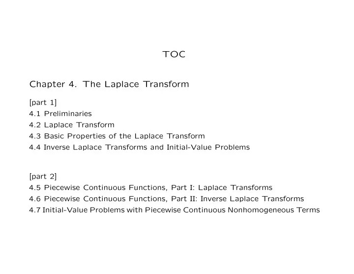
TOC Chapter 4. The Laplace Transform

[part 1] 4.1 Preliminaries 4.2 Laplace Transform 4.3 Basic Properties of the Laplace Transform 4.4 Inverse Laplace Transforms and Initial-Value Problems [part 2] 4.5 Piecewise Continuous Functions, Part I: Laplace Transforms 4.6 Piecewise Continuous Functions, Part II: Inverse Laplace Transforms 4.7 Initial-Value Problems with Piecewise Continuous Nonhomogeneous Terms

Recall: A method for solving initial-value problems for linear differential equations with constant coefficients. Can be also used if RHS is only piecewise continuous (so not continuous). F(s) = L[f(x)] :=

∞

e−sxf(x) dx Main properties:

• I. L

is linear and one-to-one

• II. L[f ′(x)] = sL[f(x)] − f(0)
• III. L[xnf(x)] = (−1)ndnF

dsn

• IV. L[f(x)] = F(s) =

⇒ L[erxf(x)] = F(s − r)

• V. (Translated Function) Let L[f(x)] := F(s) and c > 0:

L[f(x − c)u(x − c)] = e−csF(s). L−1[e−csF(s)] = f(x − c)u(x − c). where u is the Heaviside step function uc(x) = u(x − c) =

• x < c

1 x ≥ c

1

f(x) F(s) = L[f(x)] c c s, s > 0 eαx 1 s − α, s > α cos βx s s2 + β2, s > 0 sin βx β s2 + β2, s > 0 eαx cos βx s − α (s − α)2 + β2, s > α eαx sin βx β (s − α)2 + β2, s > α xn, n = 1, 2, . . . n! sn+1, s > 0 xn eαx, n = 1, 2, . . . n! (s − α)n+1, s > α x cos βx s2 − β2 (s2 + β2)2, s > 0 x sin βx 2βs (s2 + β2)2, s > 0

2

Section 4.5. Laplace Transform: Discontinuous Functions Types of discontinuities: Infinite: f(x) = 1 (x − 1)2

3

Jump: f(x) =

  

2x, 0 ≤ x < 3 4, 3 ≤ x < ∞ Removable: f(x) =

    

x2−4 x−2 ,

x = 2 1, x = 2

4

Def. Let the function f = f(x) be defined on an interval I and continuous except at a point c ∈ I. If lim

x→c− f(x)

and lim

x→c+ f(x)

exist but lim

x→c− f(x) =

lim

x→c+ f(x),

then f is said to have a jump (or finite) discontinuity at c.

5

Def. A function f defined on an interval I is piecewise continuous on I if it is continuous

• n

I except for at most a finite number of points c1, c2, . . . , cn of I at which it has jump discontinu- ities.

6

Theorem: If the function f is piecewise continuous

• n

[0, ∞), and of exponential order λ, then the Laplace transform L[f(x)] exists for s > λ.

7

Unit Step (Heaviside) Functions: Let c > 0. The function uc(x) = u(x − c) =

  

x < c 1 x ≥ c is called a unit step function.

8

Laplace Transform of a Unit Step Function: L[u(x − c)] =

∞

e−sxu(x − c) dx L[u(x − c)] = e−cs 1 s, s > 0.

9

Translation of a Function: if f is defined on [0, ∞) and c > 0, then the function f(x − c)u(x − c) =

    

0, x < c f(x − c)u(x − c), x ≥ c is the translation of f to c.

10

f(x) f(x − c)

11

f(x − c)u(x − c)

12

Translations: Express f(x) in terms of (x − c) EXAMPLES: 1. Express f(x) = 5x + 3 in terms of (x − 3) 2. Express f(x) = x2 − 3x + 7 in terms of (x − 2)

13

3. Express f(x) = sin 2x in terms of (x − π/2) 4. Express f(x) = cos πx in terms of (x − 3)

14

Property V. Laplace Transform of a Translated Function: Suppose that L[f(x)] = F(s). Then, for any positive number c, 1. L[f(x − c)u(x − c)] = e−csF(s). 2. L−1[e−csF(s)] = f(x − c)u(x − c).

15

Proof

16

Examples: Given f(x), find F(s). 1. f(x) =

  

2x, 0 ≤ x < 3 3, 3 ≤ x < ∞

17

Step 1. Re-write f in terms of u(x − 3): f(x) = 2x − 2x u(x − 3) + 3u(x − 3)

18

Graphs: 2x − 2x u(x − 3) 3u(x − 3)

19

Step 2. Write the coefficients in terms of x − 3 f(x) = 2x − 2(x − 3)u(x − 3) − 3u(x − 3)

20

Step 3. Determine L[f]: F(s) = 2 s2 − 2e−3s 1 s2 − 3e−3s 1 s

21

2. f(x) =

  

x2, 0 ≤ x < 2 3x, x ≥ 2 Step 1. Re-write f in terms of u(x − 2): f(x) = x2 − x2 u(x − 2) + 3x u(x − 2)

22

Step 2. Write the coefficients in terms of x − 2: f(x) = x2−(x−2)2u(x−2)−(x−2)u(x−2)+2u(x−2)

23

Step 3. Determine L[f]: f(x) = x2−(x−2)2u(x−2)−(x−2)u(x−2)+2u(x−2) F(s) = 2 s3 − e−2s 2 s3 − e−2s 1 s2 + 2e−2s 1 s

24

3. f(x) =

  

x + 1, 0 ≤ x < 3 sin πx, x ≥ 3 Step 1. Re-write f in terms of u(x − 3): f(x) = x + 1 − (x + 1)u(x − 3) + sin(πx) u(x − 3)

25

Step 2. Write the coefficients in terms of x − 3: f(x) = x + 1 − 4u(x − 3) − (x − 3)u(x − 3) − sin[π(x − 3)]u(x − 3)

26

Step 3. Determine L[f]: F(s) = 1 s2 + 1 s − 4e−3s1 s − e−3s 1 s2 − e−3s π s2 + π2

27

4. f(x) =

  

1 0 ≤ x < π/2 sin x π/2 ≤ x < π 2 cos x x ≥ π Step 1. Re-write f in terms of u(x − π/2) and u(x − π) :

28

Step 2. Write coefficients in terms of x − π 2 and x − π:

29

(continued) f(x) = 1 − u(x − π

2) + cos(x − π 2)u(x − π 2) + sin(x − π)u(x − π)−

2 cos(x − π)u(x − π)

30

Step 3. Determine L[f]: F(s) = 1 s − e−πs/2 1 s + e−πs/2 s s2 + 1 + e−πs 1 s2 + 1 − 2e−πs s s2 + 1

31

Section 4.6. Inverse Transforms & Piecewise Continuous Functions: Recall Property V: Suppose that L[f(x)] = F(s). Then, for any positive number c, 1. L[f(x − c)u(x − c)] = e−csF(s). 2. L−1[e−csF(s)] = f(x − c)u(x − c).

32

Examples: Given F(s), find f(x): 1. F(s) = 3 s − 2e−2s 1 s + e−2s 1 s − 2

33

Answer: f(x) = 3 − 2u(x − 2) + e2(x−2)u(x − 2) =

  

3, 0 ≤ x < 2 1 + e2(x−2), x ≥ 2

34

2. F(s) = 2 s + 4e−3s 1 s(s + 2)

35

Answer: f(x) = 2 + 2u(x − 3) − 2e−2(x−3)u(x − 3) =

    

2, 0 ≤ x < 3 4 − 2e6 e−2x, x ≥ 3

36

3. F(s) = 1 − e−πs s(s2 + 4)

37

Answer: f(x) = 1

4−1 4 cos 2x−1 4 u(x−π)+1 4 cos(2[x−π]) u(x−π)

= 1

4 − 1 4 cos 2x − 1 4 u(x − π) + 1 4 cos 2x u(x − π)

=

    

1 4 − 1 4 cos 2x,

0 ≤ x < π 0, x ≥ π .

38

4. F(s) = 4 s + 2 s2 +3e−2s1 s −2e−2s 1 s2 −5e−4s 1 s2 +e−4s 1 s − 2

39

Answer: f(x) =

          

4 + 2x, 0 ≤ x < 2 3 + 4x, 2 ≤ x < 4 23 − x + e2(x−4), x ≥ 4

40

Section 4.7. Application to Initial-Value Prob- lems with piecewise continuous RHS Examples: 1. Use the Laplace transform method to solve the initial-value problem y′ + 2y = f(x), y(0) = 1. where f(x) =

  

x 0 ≤ x < 3 1 x ≥ 3

41

Laplace transform of the solution: Y (s) = 1 s2(s + 2) − e−3s s2(s + 2) − 2 e−3s s(s + 2) + 1 s + 2 The solution: y =

            

−1 4 + 1 2 x + 5 4e−2x, 0 ≤ x < 3 1 2 + 5 4e−2x + 3 4e−2(x−3), x ≥ 3.

42

1 2 3 4 5 6 x 1 2 y

38

2. Use the Laplace transform method to solve the initial-value problem y′′ + 2y′ + y = f(x), y(0) = y′(0) = 0. where f(x) =

  

1 0 ≤ x < 2 x + 1 x ≥ 2 Laplace transform of the solution: Y (s) = 1 s(s + 1)2 + 2e−2s s(s + 1)2 + e−2s s2(s + 1)2

44

The solution: y =

    

1 − (x + 1)e−x, 0 ≤ x < 2 x − 1 − (x + 1)e−x − (x − 2)e−(x−2), x ≥ 2

45

2 x 1 2 3 y

41