Landmark Map L11: Landmark Mapping Locations and uncertainties of - - PDF document

1

L11: Landmark Mapping

CS 344R/393R: Robotics Benjamin Kuipers

Landmark Map

• Locations and uncertainties of n landmarks,

with respect to a specific frame of reference.

– World frame: fixed origin point – Robot frame: origin at the robot

• Problem: how to combine new information

with old to update the map.

A Spatial Relationship is a Vector

• A spatial relationship holds between two

poses: the position and orientation of one, in the frame of reference of the other.

xAB = xAB yAB AB

• xAB = xAB

yAB AB

[ ]

T

A B

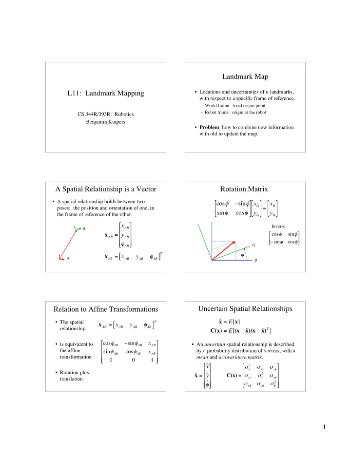
Rotation Matrix

cos sin sin cos

• xG

yG

• = xB

yB

• B

G

cos sin sin cos

• Inverse:

Relation to Affine Transformations

• The spatial

relationship

• is equivalent to

the affine transformation

• Rotation plus

translation

xAB = xAB yAB AB

[ ]

T

cosAB sinAB xAB sinAB cosAB yAB 1

• Uncertain Spatial Relationships
• An uncertain spatial relationship is described

by a probability distribution of vectors, with a mean and a covariance matrix.

ˆ x = E[x] C(x) = E[(x ˆ x )(x ˆ x )T ] ˆ x = ˆ x ˆ y ˆ

• C(x) =

x

2

xy x xy y

2

y x y

• 2

2

A Map with n Landmarks

• Concatenate n vectors into one big state vector
• And one big 3n×3n covariance matrix.

x = x1 x2 M xn

• ˆ

x = ˆ x

1

ˆ x

2

M ˆ x

n

• C(x) =

C(x1) C(x1,x2) L C(x1,xn) C(x2,x1) C(x2) L C(x2,xn) M M O M C(xn,x1) C(xn,x2) L C(xn)

• Example
• The robot senses object #1.
• The robot moves.
• The robot senses a different object #2.
• Now the robot senses object #1 again.
• After each step, what does the robot know

(in its landmark map) about each object, including itself?

Robot Senses Object #1 and Moves Robot Senses Object #2 Robot Senses Object #1 Again Updated Estimates After Constraint

3

Compounding

xAB = xAB yAB AB

[ ]

T

xBC = xBC yBC BC

[ ]

T

Compounding

xAB = xAB yAB AB

[ ]

T

xBC = xBC yBC BC

[ ]

T

xAC = xAC yAC AC

[ ]

T

Compounding

• Let xAB be the pose of object B in the frame
• f reference of A. (Sometimes written BA.)
• Given xAB and xBC, calculate xAC.
• Compute C(xAC) from C(xAB), C(xBC), and

C(xAB,xBC).

xAC = xAB xBC = xBC cosAB yBC sinAB + xAB xBC sinAB + yBC cosAB + yAB AB + BC

• Computing Covariance
• Apply this to nonlinear functions by using

Taylor Series.

y = Mx + b C(y) = C(Mx + b) = E[(Mx + b (Mˆ x + b)) (Mx + b (Mˆ x + b))T] = E[M(x ˆ x ) (M(x ˆ x ))T] = E[M (x ˆ x )(x ˆ x )T MT] = M E[(x ˆ x )(x ˆ x )T ]MT = MC(x)MT

• Consider the linear mapping y = Mx+b

Inverse Relationship

xAB = xAB yAB AB

[ ]

T

xBA = xBA yBA BA

[ ]

T

The Inverse Relationship

• Let xAB be the pose of object B in the frame
• f reference of A.
• Given xAB, calculate xBA.
• Compute C(xBA) from C(xAB)

xBA = ()xAB = xAB cosAB yAB sinAB xAB sinAB yAB cosAB AB

4

Composite Relationships

• Compounding combines relationships head-

to-tail: xAC = xAB ⊕ xBC

• Tail-to-tail combinations come from
• bserving two things from the same point:

xBC = (xAB) ⊕ xAC

• Head-to-head combinations come from two
• bservations of the same thing:

xAC = xAB ⊕ (xCB)

• They provide new relationships between

their endpoints.

Merging Information

• An uncertain observation of a pose is

combined with previous knowledge using the extended Kalman filter.

– Previous knowledge: – New observation: zk, R

• Update: x = x(new) ⊗ x(old)
• Can integrate dynamics as well.

xk

,

Pk

• EKF Update Equations
• Predictor step:
• Kalman gain:
• Corrector step:

ˆ x

k = f (ˆ

x

k1,uk )

Pk

= APk1A T + Q

K k = P

k H T (HPk H T + R) 1

ˆ x

k = ˆ

x

k + Kk(zk h(ˆ

x

k ))

Pk = (IK kH)Pk

• Reversing and Compounding
• OBJ1R = (ROBOTW) ⊕ OBJ1W
• = WORLDR ⊕ OBJ1W

Sensing Object #2

• OBJ2W = ROBOTW ⊕ OBJ2R

Observing Object #1 Again

• OBJ1W = ROBOTW ⊕ OBJ1R

5

Combining Observations (1)

• OJB1W = OJB1W(new) ⊗ OBJ1W(old)
• OJB1R = OJB1R(new) ⊗ OBJ1R(old)

Combining Observations (2)

• ROBOTW(new) = OJB1W ⊕ (OBJ1R)
• ROBOTW = ROBOTW(new) ⊗ ROBOTW(old)

Useful for Feature-Based Maps

• We’ll see this again when we study

FastSLAM.