Kpax Protein Structure Alignment Demo: Using Kpax on Linux Dave - - PowerPoint PPT Presentation

Kpax – Protein Structure Alignment

Dave Ritchie

Team Orpailleur Inria Nancy – Grand Est

Outline

Overview of Protein Sequences and Structures Structural Alignment Using Dynamic Programming The Kpax Algorithm Explained Demo: Using Kpax on Linux Practical: Homology Modeling Using Kpax + Modeler

2 / 33

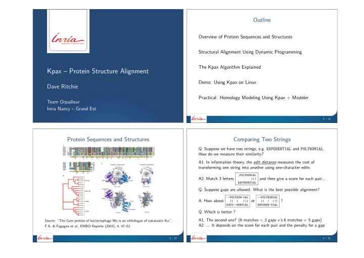
Protein Sequences and Structures

Source: ”The Gam protein of bacteriophage Mu is an orthologue of eukaryotic Ku”, F.A. di Fagagna et al., EMBO Reports (2003), 4, 47–52

3 / 33

Comparing Two Strings

• Q. Suppose we have two strings, e.g. EXPONENTIAL and POLYNOMIAL.

How do we measure their similarity?

• A1. In information theory, the edit distance measures the cost of

transforming one string into another using one-character edits

• A2. Match 3 letters

POLYNOMIAL ||| EXPONENTIAL

and then give a score for each pair...

• Q. Suppose gaps are allowed. What is the best possible alignment?
• A. How about
• -POLYNOM-IAL

|| | ||| EXPO--NENTIAL

• r
• -POLYNOMIAL

|| | ||| EXPONEN-TIAL

?

• Q. Which is better ?
• A1. The second one? (6 matches + 3 gaps v’s 6 matches + 5 gaps)
• A2. ... It depends on the score for each pair and the penalty for a gap

4 / 33

Dynamic Programming

Dynamic programming (DP) is a method of dividing a problem into smaller sub-problems. It was first described by Richard Bellman in the 1940s. But instead of using recursion, it uses a table (“memoisation” in 1940s language).

Goal: find similarity E(n, m) between two strings: x[1:n] and y[1:m] Sub-goal: find E(i, j) between two prefixes: x[1:i] and y[1:j] Observation: the best alignment must end on

x[i] y[j] or x[i] −

• r

− y[j]

Method: build similarity table with scores S(i, j) and penalties P(i):

E(i, j) = max      E(i − 1, j − 1) + S(i, j) E(i, j − 1) − P(i) E(i − 1, j) − P(j)

Then, “trace back” from E(n, m) to E(1, 1) to extract the alignment

5 / 33

Back-Tracking Through The DP Scoring Table

E X P O N E N T I A L 1 2 3 4 5 6 7 8 9 10 11 12 P O L Y N O M I A L p p p p p p p p p p p p p p p p p p p p p p p p 0 1 2 3 4 5 6 7 8 9 1011

This gives the desired optimal alignment

• -POLYNOMIAL

|| | ||| EXPONEN-TIAL

6 / 33

3D Least-Squares Fitting

Least-squares fitting finds the 3D rotation/translation matrix M that minimises the sum of squared distances: F =

N

• i=1

(xA

i − M.xB i )2

For proteins, the xi are normally Cα atom coordinates The translational part is easy – shift centres of mass to the origin The rotation can be found using eigenvector or quaternion methods The residual error (RMSD) is then given by RMSD =

• 1

N

N

• i=1

(xA

i − M.xB i )2

So, given list of aligned Cα’s, we can fit optimally to some RMSD

7 / 33

So, What’s The Problem?

DP is “perfect” for 1D string matching Least-squares fitting is “perfect” for 3D superposition BUT Proteins are not made of 1D symbols or 3D points. They are made

• f complex 3D chemical components (amino acid residues). It is

difficult to write a good scoring function to compare residues... Similar 1D protein sub-sequences can have different 3D shapes (α-helices, β-strands), i.e. global environment can affect local shape. We don’t know a priori the right 1D pairings for 3D fitting... Proteins are globally flexible. Even if many local 1D regions “match”, not all of them might simultaneously superpose well in 3D space... ADDITIONALLY! Proteins can contain multiple repeats and/or transpositions...

8 / 33

Over 100 Structure Alignment Algorithms in 25 Years

http://en.wikipedia.org/wiki/Structural alignment software 90 more...

9 / 33

Quick List of Structural Alignment Approaches

“elastic” Gaussian scoring “double dynamic programming” on Cα distance matrices triples or higher fragments (8-tuples) of Cα atoms backbone Cα vectors backbone torsion angles secondary structure elements geometric hashing Voronoi tessellations structural alphabets Lagrangian contact map optimisation eigenvector analysis of distance matrices Fourier correlations Gaussian fragments ...

10 / 33

Introducing Kpax

http://kpax.loria.fr/ Dynamic programming with Gaussian scores Uses NO sequence similarity OR secondary structure information Very fast database search (CATH, SCOP, Pfam, ..., user-defined) Rigid and flexible structural alignments Multiple flexible alignments coming soon...

11 / 33

Defining Local Coordinate Frames

All Cα atoms have highly conserved tetrahedral geometry

Exploit this to define a “canonical” Cα–C–N orientation e.g. put Cα at origin; C on -ve z axis; N in +ve xz plane

Now, ALL α-helices and β-strands look the same at the origin

12 / 33

Comparing Structural Fragments

In the canonical frame, similar structures have similar distances between their up-stream and down-stream Cαatoms: But how to combine all the distances into a single score?

13 / 33

Representing Local Geometry as a Product of Gaussians

Calculate Gaussian distribution of all Cα atoms in CATH

CATH

• 3
• 2
• 1

+1 +2 +3 y z x

Gives Gaussian width σk for each up-stream and down-stream Cα Then, represent residue i as a product of Gaussians: ψi = φ−1

i

(xi−1)φ+1

i

(xi+1) ... φ−n

i

(xi−n)φ+n

i

(xi+n) each individual Gaussian function has the form: φk

i (xi+k) = Nke−βkr2

k /2σ2 k 14 / 33

Calculating a Per-Residue Local Similarity Score

Calculate the local-frame similarity, K local

ij

, as an overlap integral K local

ij

=

• ψiψj dx−n...+n.

With products of Gaussians, this reduces to a simple sum K local

ij

= e− n

k=−n βkR2 i+k,j+k/4σ2 k,

In identical α-helices, β-strands, and even loops, K local

ij

= 1.

15 / 33

Detecting Secondary Structure Elements

By sliding a model α-helix and β-strand along a structure, Kpax detects its secondary structure elements (SSEs) automatically (it does not distinguish π or 310 helices or detect β-turns). Here are some examples: Nice, but how to match correctly a short α-helix with a longer one?

16 / 33

The Spatial Similarity Score

If two similar protein domains are superposed, their centres of mass (COM) will be close together. Therefore, in the local coordinate frame, well-aligned residues will “see” the COM in similar positions in space (but consecutive residues will see the COM in quite different positions).

From the COM direction vector, we get a spatial similarity score K spatial

ij

= e− n

k=−n βkR2 i+k,j+k/4τ 2 k 17 / 33

The Kpax Structure Alignment Algorithm

The “local” and “spatial” scores give a kind of “1D preview” of how two proteins might be aligned without actually moving them K 1D

ij

= (K local

ij

+ K spatial

ij

)/2 Once the proteins are superposed, we can calculate real 3D Gaussian overlap scores for every pair of residues: G3D

ij

= e−R2

ij/4τ 2

This leads to the following algorithm:

1 Set per-residue gap penalties according to SSE types 2 Apply DP to the K-scores to get the first correspondence 3 Fit some/all fragments by least-squares and superpose 4 Calculate 3D G-scores between close pairs of residues 5 Apply DP to the G-scores to get a new correspondence 18 / 33

Generating Fitting Fragments From The K-Scores

Blocks of high K-scores arise when SSEs detect each other:

γ α α γ β β β γ α α γ γ α α γ β β β γ α α pγ pα pα pγ pβ pβ pβ pγ pα pα pγ pγpαpαpγpβpβpβpγpαpα 0

The alignment: —

γ | γ — αα | | αα

—

γ | γ — βββ | | | βββ — γ | γ — αα | | αα

—

• |

γ —

Next, use the pairs within each blue block as fitting candidates... (γ means “loop”)

19 / 33

Scoring Trial Superpositions Using G-Scores

Evaluate each trial superposition using real 3D coordinates (G-scores):

0 0 0 0 0 0 0 0 0 0 0

The aligned residues: —

γγγ AGQ ||| LPD

—

αααα LLADA ||||| LKVYA

—

γγ QN || QR

—

ββββββ RGDYWSD ||||||| GADFWLA

— ------PDAGV

QRSLKV-----

— (no gap penalties)

20 / 33

Example 1: Aligning Ubiquitin and Ferrodoxin I

TM-Align: 63 residues aligned, Cα RMSD = 2.6˚ A Kpax-1.0: 45 residues aligned, Cα RMSD = 2.0˚ A My claim: Kpax gives a tighter alignment than TM-Align

21 / 33

Example 2: methyl dehydroxygenase / galactose oxidase

The SCOP domains d4aaha and d1gofa3

TM-Align: 336 residues aligned, CαRMSD = 5.4˚ A Kpax-1.0: 178 residues aligned, CαRMSD = 3.9˚ A Difference: 11.6 ˚ A RMSD

... I believe the Kpax alignment is correct!

22 / 33

Building and Searching Structural Databases

Before calculating an alignment, Kpax pre-processes each protein

• separately. The pre-processed data can be stored to make a

structural database... NB. It takes more time to read a PDB file than to do an alignment ! Shift the protein to put its COM at the world origin Calculate 6 local and 6 spatial “atom” coordinates per residue Determine the SSE type of each residue Save this data and original PDB coords as binary “blobs” Use Linux “memory mapping” to read a binary database Use Posix threads to do all calculations in parallel Result: Searching 11,000 CATH structures takes about 4 seconds...

23 / 33

ROC-Plot Comparison with TM-Align and Yakusa

We selected 213 CATH families, each having ≥ 10 members Searched CATH database with one structure from each family

TP (true pos) when [C.A.T.H] code of query matches database FP (false pos) when query matches some other CATH code

0.0 0.2 0.4 0.6 0.8 1.0 0.0 0.2 0.4 0.6 0.8 1.0 False positive rate True positive rate TM−Align Kpax Yakusa random

TM-align AUC = 0.976, Kpax AUC = 0.966, Yakusa AUC = 0.915 TM-align 46 h; Yakusa 2.2 h; Kpax 0.3h (i.e. Kpax is 150x / 6x faster)

24 / 33

Flexible Alignment – Finding More Fitting Fragments

For flexible alignment, just fill in the remaining boxes:

γ α α γ γ α α 0 pγpαpα 0 pγ pα pα pγ

Candidate fitting fragments: —

γ | γ — αα | | αα

—

• |

γ —

25 / 33

The Final Flexible Alignment

After a further round of DP, we get the final “flexible” alignment:

0 0 0 0 0 0 0 0 0 0 0

• NB. the 3D structure may have discontinuities between the fitted segments:

—

γγγ AGQ ||| LPD

—

αααα LLADA ||||| LKVYA

—

γγ QN || QR

—

ββββββ RGDYWSD ||||||| GADFWLA

–?–

γ P | Q

—

ααα DAG ||| RSL

—

γγ

• V

| KV

—

26 / 33

Example 1 Revisited – Flexible Kpax

ubiquitin (green) and ferrodoxin I (blue)

Kpax-1.0: 45 residues aligned, Cα RMSD = 2.0˚ A (rigid) Kpax-2.2: 57 residues aligned, Cα RMSD = 2.8˚ A (rigid) Kpax-2.2: 56 residues aligned, Cα RMSD = 2.2˚ A (flexible)

Rigid superposition: white = anchor; yellow = aligned Flex superposition: (re-fitted anchors, new segment in orange)

27 / 33

Example 2 Revisited – Flexible Kpax

d4aaha and d1gofa3 (looking directly at the β-propeller)

Kpax-1.0: 178 residues aligned, CαRMSD = 3.9˚ A (rigid) Kpax-2.2: 218 residues aligned, CαRMSD = 3.2˚ A (rigid) Kpax-2.2: 260 residues aligned, CαRMSD = 1.7˚ A (flexible)

Rigid superposition: white = anchor; yellow = aligned Flex superposition: 20 segments (anchor in white)

28 / 33

Aligning Human and Fly Calmodulin

Calmodulin (Ca-binding protein) is found in all eukaryotic cells

Green = 1CLL (human: homo sapiens) Blue = 2BBM (fly: dropsophila melanogaster) Both superpositions have 4 segments (137 residues, 1.7 ˚ A RMSD)

29 / 33

Human Blood Factor and a Parasite Surface Protein

Green = 1DAN (human blood coagulation factor VIIA) Blue = 1B9W (Plasmodium cynomolgi merozoite surface protein) 4/4 segments, 70/77 residues, 18/19 identities, 1.8/1.9 ˚ A RMSD

30 / 33

Multiple Flexible Alignments and Modeling

Multiple Structural Alignments (unpublished)

Kpax 4.0 uses “pile-up” method for multiple alignments Choose “centre” or “pivot” structure; fit the rest on to it Also works with flexible alignments to the pivot

Automatic Homology Modeling Pipeline (unpublished)

Use a protein sequence as the search query... ... find the structure with the closest sequence and use as “pivot” Perform a structural search using pivot as query... ... make multiple structural alignment of closest hits Generate Modeler command script automatically :-)

Worked Example – Cyp450

kpax -db=cyp450 -model -show=20 my secret cyp.fasta

31 / 33

Conclusion and Future Prospects

Conclusions Tight high quality structural alignments Fast structural databases searches Flexible alignments now possible Multiple alignments now possible All-versus-all structural comparisons now possible Future Prospects Better structural alignments → better holomology models... Should help study evolutionary relationships at structural level ...

32 / 33

Thank You! Acknowledgments

Anisah Ghoorah Lazaros Mavridis Vishwesh Venkatraman April Chung Niruba Thiagarajan

33 / 33

Program and paper:

http://kpax.loria.fr/

Kpax Demo – Basic Operations

Download Kpax from: http://kpax.loria.fr/download-3.2-beta/ Example pairs of structures: http://hex.loria.fr/emmsb/kpax examples/

Aligning two structures Viewing the results in Hex and VMD Performing flexible structural alignments Building and searching a structural database Performing multiple structural alignments Viewing multiple alignments in Hex/VMD ... Ask me! Disclaimer: Kpax is not “commercial” software!

34 / 33

Practical Activities – 1

Downloading the data

Download the API-A sequence from: http://hex.loria.fr/emmsb/t40.tgz t40 c.fasta (API-A) Download the CATH database from: http://hex.loria.fr/emmsb/cath/ CathDomainPdb.S35.v3 4 0.tgz (260 Mb of compressed PDB files) CathDomainList.gz (1.3 Mb file of CATH codes) build cath.sh (shell script to build a Kpax database)

Building a Kpax database

Unzip the two zip files (use gunzip) Edit the script to have the correct path to the data (CATH ROOT=???) Run the script to build that database (takes a few minutes) Run kpax with -help option to show all the parameters and options; try: kpax -db=cath -list

35 / 33

Practical Activities – 2

Searching a database and visualising the results

Try searching the database with t40 c.pdb as the query Go to the results folder (kpax results/t40 c) and look at the results files Use Hex or VMD to visualise the results (.mac for Hex and .tcl for VMD) Do you agree with the superpositions?

Making a MSA for homology modeling

Run kpax to make a multiple structure alignment from the seed sequence The command for this is of the form: kpax -db=cath -model -top=24 t40 c.fasta cd to the results folder (kpax results/2qn4A00) and examine the contents

Making a homology model (optional)

Run Modeler (the actual command may differ on your machine):

/opt/modeller/bin/mod9.13 t40 c modeller.py

Use Kpax/Hex to compare the model and real structure (t40 c.pdb)

36 / 33