VI.3 Rule-Based Information Extraction Goal: Identify and extract - - PowerPoint PPT Presentation

vi 3 rule based information extraction
SMART_READER_LITE
LIVE PREVIEW

VI.3 Rule-Based Information Extraction Goal: Identify and extract - - PowerPoint PPT Presentation

VI.3 Rule-Based Information Extraction Goal: Identify and extract unary, binary, or n -ary relations as facts embedded in regularly structured text , to generate entries in a schematized database Rule-driven regular expression matching


slide-1
SLIDE 1

IR&DM ’13/’14

VI.3 Rule-Based Information Extraction

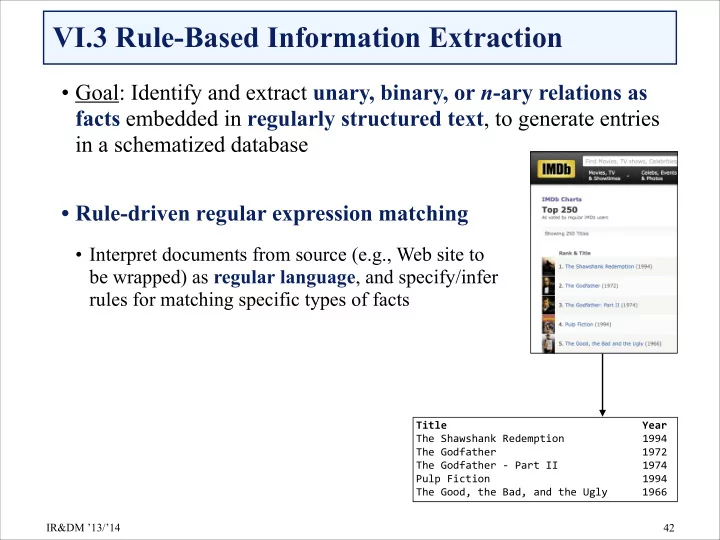
  • Goal: Identify and extract unary, binary, or n-ary relations as

facts embedded in regularly structured text, to generate entries in a schematized database


  • Rule-driven regular expression matching
  • Interpret documents from source (e.g., Web site to


be wrapped) as regular language, and specify/infer
 rules for matching specific types of facts

!42 Title& & & & & & & Year& The%Shawshank%Redemption% % % 1994% The%Godfather% % % % % 1972% The%Godfather%C%Part%II% % % 1974% Pulp%Fiction% % % % % 1994% The%Good,%the%Bad,%and%the%Ugly% % 1966

slide-2
SLIDE 2

IR&DM ’13/’14

LR Rules

  • L token (left neighbor) fact token

R token (right neighbor)
 pre-filler pattern filler pattern post-filler pattern


  • Example:


L = <B>, R = </B>
 → Country
 L = <I>, R = </I>
 → Code
 produces relation with
 tuples <Congo,%242>,%<Egypt,%20>,%<France,%30>


  • Rules are often very specific and therefore combined/generalized
  • Full details: RAPIER [Califf and Mooney ’03]

!43

<HTML>% % <TITLE>Some%Country%Codes</TITLE>%% <BODY>% % <B>Congo</B><I>242</I><BR>% % <B>Egypt</B><I>20</I><BR>% % <B>France</B><I>30</I><BR>% </BODY>% </HTML>

slide-3
SLIDE 3

IR&DM ’13/’14

Advanced Rules: HLRT, OCLR, NHLRT, etc.

  • Idea: Limit application of LR rules to proper context


(e.g., to skip over HTML table header)


  • HLRT rules (head left token right tail)


apply LR rule only if inside HT (e.g., H = <TD> T = </TD>)

  • OCLR rules (open (left token right)* close):


O and C identify tuple, LR repeated for individual elements

  • NHLRT (nested HLRT):


apply rule at current nesting level,


  • pen additional levels, or return to higher level

!44

<TABLE>% & <TR><TH><B>Country</B></TH><TH><I>Code</I></TH></TR>& & <TR><TD><B>Congo</B></TD><TD><I>242</I></TD></TR>& & <TR><TD><B>Egypt</B></TD><TD><I>20</I></TD></TR>& & <TR><TD><B>France</B></TD><TD><I>30</I></TD></TR>& </TABLE>

slide-4
SLIDE 4

IR&DM ’13/’14

Learning Regular Expressions

  • Input: Hand-tagged examples of a regular language
  • Learn: (Restricted) regular expression for the language of a finite-state

transducer that reads sentences of the language and outputs token of interest

  • Example:


 This apartment has 3 bedrooms. <BR> The monthly rent is $ 995.
 This apartment has 4 bedrooms. <BR> The monthly rent is $ 980.
 The number of bedrooms is 2. <BR> The rent is $ 650 per month.
 
 yields * <digit> * “<BR>” * “$” <digit>+ * as learned pattern

  • Problem: Grammar inference for full-fledged regular languages is hard.

Focus therefore often on restricted class of regular languages.


  • Full details: WHISK [Soderland ’99]


!45

slide-5
SLIDE 5

IR&DM ’13/’14

Properties and Limitations of Rule-Based IE

  • Powerful for wrapping regularly structured web pages


(e.g., template-based from same deep web site)


  • Many complications with real-life HTML


(e.g., misuse of tables for layout)


  • Flat view of input limits the same annotation
  • Consider hierarchical document structure (e.g., DOM tree, XHTML)
  • Learn extraction patterns for restricted regular languages


(e.g., combinations of XPath and first-order logic)


  • Regularities with exceptions are difficult to capture
  • Learn positive and negative cases (and use statistical models)

!46

slide-6
SLIDE 6

IR&DM ’13/’14 IR&DM ’13/’14 IR&DM ’13/’14

Additional Literature for VI.3

  • M. E. Califf and R. J. Mooney: Bottom-Up Relational Learning of Pattern Matching

Rules for Information Extraction, JMLR 4:177-210, 2003

  • S. Soderland: Learning Information Extraction Rules for Semi-Structured and Free

Text, Machine Learning 34(1-3):233-272, 1999

!47

slide-7
SLIDE 7

IR&DM ’13/’14

VI.4 Learning-Based Information Extraction

  • For heterogeneous sources and for natural-language text
  • NLP techniques (PoS tagging, parsing) for tokenization
  • Identify patterns (regular expressions) as features
  • Train statistical learners for segmentation and labeling


(e.g., HMM, CRF, SVM, etc.) augmented with lexicons

  • Use learned model to automatically tag new input sequences
  • Training data:


The WWW conference takes place in Banff in Canada
 Today’s keynote speaker is Dr. Berners-Lee from W3C
 The panel in Edinburgh chaired by Ron Brachman from Yahoo!


 with event, location, person, and organization annotations

!48

slide-8
SLIDE 8

IR&DM ’13/’14

IE as Boundary Classification

  • Idea: Learn classifiers to recognize start token and end token for

the facts under consideration. Combine multiple classifiers (ensemble learning) for more robust output.


  • Example:


There will be a talk by Alan Turing at the University at 4 PM.


  • Prof. Dr. James Watson will speak on DNA at MPI at 6 PM.


 The lecture by Francis Crick will be in the IIF at 3 PM.

!

  • Classifiers test each token (with PoS tag, LR neighbor tokens, etc.

as features) for two classes: begin-fact, end-fact


!49

person place time

slide-9
SLIDE 9

IR&DM ’13/’14

Text Segmentation and Labeling

  • Idea: Observed text is concatenation of structured record with

limited reordering and some missing fields


  • Example: Addresses and bibliographic records


  • Source: [Sarawagi ’08]

!50

Page Volume Author Year Title Journal

4089 Whispering Pines Nobel Drive San Diego CA 92122 P.P.Wangikar, T.P. Graycar, D.A. Estell, D.S. Clark, J.S. Dordick (1993) Protein and Solvent Engineering of Subtilising BPN' in Nearly Anhydrous Organic Media J.Amer. Chem. Soc. 115, 12231-12237.

House number Building Road City Zip State

slide-10
SLIDE 10

IR&DM ’13/’14

Hidden Markov Models (HMMs)

  • Assume that the observed text is generated by a regular grammar


with some probabilistic variation (i.e., stochastic FSA = Markov Model)


  • Each state corresponds to a category (e.g., noun, phone number, person)


that we seek to label in the observed text


  • Each state has a known probability distribution over words


that can be output by this state


  • The objective is to identify the state sequence (from a start to an end state)

with maximum probability of generating the observed text


  • Output (i.e., observed text) is known, but the state sequence cannot be
  • bserved, hence the name Hidden Markov Model 


!51

slide-11
SLIDE 11

IR&DM ’13/’14

Hidden Markov Models

  • Hidden Markov Model (HMM) is a 


discrete-time, finite-state Markov model consisting of

  • state space S = {s1, …, sn} and the state in step t is denoted as X(t)
  • initial state probabilities pi (i = 1, …, n)
  • transition probabilities pij : S × S → [0,1], denoted p(si → sj)
  • output alphabet Σ = {w1, …, wm}
  • state-specific output probabilities qik : S × Σ → [0,1], denoted q(si ↑ wk)

  • Probability of emitting output sequence o1, …, oT ∈ ΣT 


 with p(x0 → xi) = p(xi)

!52

X

x1,...,xT ∈S T

Y

i=1

p(xi−1 → xi) q(xi ↑ oi)

slide-12
SLIDE 12

IR&DM ’13/’14

HMM Example

  • Goal: Label the tokens in the sequence


Max-Planck-Institute, Stuhlsatzenhausweg 85
 with the labels Name, Street, Number
 
 Σ = {“MPI”, “St.”, “85”} // output alphabet
 S = {Name, Street, Number} // (hidden) states
 pi = {0.6, 0.3, 0.1} // initial state probabilities

!53

Start Name Street End Number

“MPI” “St.” “85”

0.1 0.3 0.6 0.2 0.4 0.1 0.5 0.4 0.1 0.2 0.4 0.4 0.7 0.2 0.8 1.0 0.3 0.3

slide-13
SLIDE 13

IR&DM ’13/’14

Three Major Issues with HMMs

  • Compute probability of output sequence for known parameters
  • Forward/Backward computation

  • Compute most likely state sequence 


for given output and known parameters (decoding)

  • Viterbi algorithm (using dynamic programming)

  • Estimate parameters (transition probabilities and output

probabilities) from training data (output sequences only)

  • Baum-Welch algorithm (specific form of Expectation Maximization)

!

  • Full details: [Rabiner ’90]

!54

slide-14
SLIDE 14

IR&DM ’13/’14

Forward Computation

  • Probability of emitting output sequence o1, …, oT ∈ ΣT is


 with p(x0 → xi) = p(xi)


  • Naïve computation would require O(nT) operations!
  • Iterative forward computation with clever caching and reuse of

intermediate results (“memoization”) requires O(n2 T) operations

  • Let αi(t) = P[o1, …, ot-1, X(t) = i] denote the probability of being in state i


at time t and having already emitted the prefix output o1, …, ot-1

  • Begin:
  • Induction:

!55

X

x1,...,xT ∈S T

Y

i=1

p(xi−1 → xi) q(xi ↑ oi) αi(1) = pi αj(t + 1) =

n

X

i=1

αi(t) p(si → sj) p(si ↑ ot)

slide-15
SLIDE 15

IR&DM ’13/’14

Backward Computation

  • Probability of emitting output sequence o1, …, oT ∈ ΣT is


 with p(x0 → xi) = p(xi)


  • Naïve computation would require O(nT) operations!
  • Iterative backward computation with clever caching and reuse
  • f intermediate results (“memoization”)
  • Let βi(t) = P[ot+1, …, oT, X(t) = i] denote the probability of being in state i


at time t and having already emitted the suffix output ot+1, …, oT

  • Begin:
  • Induction:

!56

X

x1,...,xT ∈S T

Y

i=1

p(xi−1 → xi) q(xi ↑ oi) βi(T) = 1 βj(t − 1) =

n

X

i=1

βi(t) p(sj → si) p(si ↑ ot)

slide-16
SLIDE 16

IR&DM ’13/’14

Trellis Diagramm for HMM Example

  • Forward probabilities:


αName (1) = 0.6 
 αStreet (1) = 0.3 
 αNumber (1) = 0.1 
 
 αName (2) = 0.6 * 0.7 * 0.2 + 0.3 * 0.2 * 0.2 + 0.1 * 0.0 * 0.1
 = 0.096

!57

Start

Name Street

End

Number

“MPI” “St” “85”

Name Street

Number

Name Street

Number

t=1 t=2 t=3

Start Name Street End Number

“MPI” “St.” “85”

0.1 0.3 0.6 0.2 0.4 0.1 0.5 0.4 0.1 0.2 0.4 0.4 0.7 0.2 0.8 1.0 0.3 0.3

slide-17
SLIDE 17

IR&DM ’13/’14

Larger HMM for Bibliographic Records

  • Source: [Chakrabarti ’09]

!58

slide-18
SLIDE 18

IR&DM ’13/’14

Viterbi Algorithm

  • Goal: Identify state sequence x1, …, xT most likely of having

generated the observed output o1, …, oT

  • Viterbi algorithm (dynamic programming)


 // highest probability of being in state i at step 1
 // highest-probability predecessor of state i
 
 for t = 1, …, T
 
 // probability
 
 // state


  • Most likely state sequence can be obtained by means of

backtracking through the memoized values δi (t) and ψi (t)

!59

δi(1) = pi ψi(1) = 0 δj(t + 1) = max

i=1, ..., n δi(t) p(xi → xj) q(xi ↑ ot)

ψj(t + 1) = arg max

i=1, ..., n

δi(t) p(xi → xj) q(xi ↑ ot)

slide-19
SLIDE 19

IR&DM ’13/’14

Training of HMMs

  • Simple case: If fully tagged training sequences are available, we

can use MLE to estimate the parameters


! !

  • Standard case: Training with unlabeled sequences 


(i.e., observed output only, state sequence is unknown)

  • Baum-Welch algorithm (variant of Expectation Maximization)

  • Note: There exists some work on learning the structured of HMMs


(# states, connections, etc.), but this remains very difficult and
 computationally expensive

!60

p(si → sj) = # transitions si → sj P

sk # transitions si → sk

q(si → wk) = # outputs si → wk P

wl # outputs si → wl

slide-20
SLIDE 20

IR&DM ’13/’14

Problems and Extensions of HMMs

  • Individual output letters/words may not show learnable patterns
  • output words can be entire lexical classes (e.g., numbers, zip code, etc.)
  • Geared for flat sequences, not for structured text documents
  • use nested HMMs where each state can hold another HMM

  • Cannot capture long-range dependencies (Markov property)


(e.g., in addresses: with first word being “Mr.” or “Mrs.”, the probability of seeing a P.O. box later decreases substantially)

  • Cannot easily incorporate multiple complex word features


(e.g., isYear(w), isDigit(w), allCaps(w), etc.)

  • Conditional Random Fields (CRFs) address these limitations

!61

slide-21
SLIDE 21

IR&DM ’13/’14 IR&DM ’13/’14 IR&DM ’13/’14

Additional Literature for VI.4

  • S. Chakrabarti: Extracting, Searching, and Mining Annotations on the Web, Tutorial,


WWW 2009 (http://www2009.org/pdf/T10-F%20Extracting.pdf)

  • L. R. Rabiner: A Tutorial on Hidden Markov Models and Selected Applications in

Speech Recognition, Readings in Speech Recognition, 1990

!62

slide-22
SLIDE 22

IR&DM ’13/’14

VI.5 Named Entity Reconciliation

  • Problem 1: Same entity appears in
  • Different spellings (incl. misspellings, abbreviations, etc.)


(e.g., brittnee spears vs. britney spears)

  • Different levels of completeness


(e.g., joe hellerstein vs . prof. joseph m. hellerstein)

  • Problem 2: Different entities happen to look the same


(e.g., george w. bush vs. george h. w. bush)


  • Problems even occur in structured databases and require 


data cleaning when integrating multiple databases

  • Integrating heterogeneous databases or Deep Web sources also


requires schema matching (aka. data integration)

!63

slide-23
SLIDE 23

IR&DM ’13/’14

Entity Reconciliation Techniques

  • Edit distance measures (both strings and records)
  • Exploit context information for higher-confidence matchings


(e.g., publications/co-authors of Dave Dewitt and D. J. DeWitt)

  • Exploit reference dictionaries as ground truth


(e.g., for address cleaning)

  • Propagate matching confidence values


in link-/reference-based graph structure

  • Statistical learning in (probabilistic) graphical models


(also: joint disambiguation of multiple mentions onto most compact/consistent set of entities)

!64

slide-24
SLIDE 24

IR&DM ’13/’14

Entity Reconciliation by Matching Functions

  • Fellegi-Sunter Model as framework for entity reconciliation


Input: Two sets A and B of strings or records
 each with features (e.g., n-grams, attributes, etc.)

  • Method:
  • Define family γi : A × B → {0,1} (i = 1, …, k)

  • f attribute comparisons or similarity tests (aka. matching functions)
  • Identify matching pairs M ⊆ A × B and non-matching pairs U ⊆ A × B


as training data and compute mi = P[γi (a,b) = 1 | (a,b) ∈ M] and 
 ui = P[γi (a,b) = 1 | (a,b) ∈ U]

  • For pairs (a,b) ∈ A × B \ (M ∪ U), consider a and b equivalent if


 for user-defined threshold τ


  • Full details: [Fellegi and Sunter ’69]

!65

k

X

i=1

mi ui · γi(a, b) ≥ τ

slide-25
SLIDE 25

IR&DM ’13/’14 IR&DM ’13/’14 IR&DM ’13/’14

  • I. Fellegi and A. Sunter: A Theory for Record Linkage, Journal of the American

Statistical Association 64(328):1183-1210, 1969

Additional Literature for VI.5

!66