
SLIDE 1
1
Announcements
- Since Thursday we’ve been discussing
chapters 7 and 8.
- “matlab can be used off campus by logging into your
wam account and bringing up an xwindow and running "tap matlab" to find out the command to run matlab which will bring it up in the xwindow.”
Edge is Where Change Occurs
- Change is measured by derivative in 1D
- Biggest change, derivative has
maximum magnitude
- Or 2nd derivative is zero.
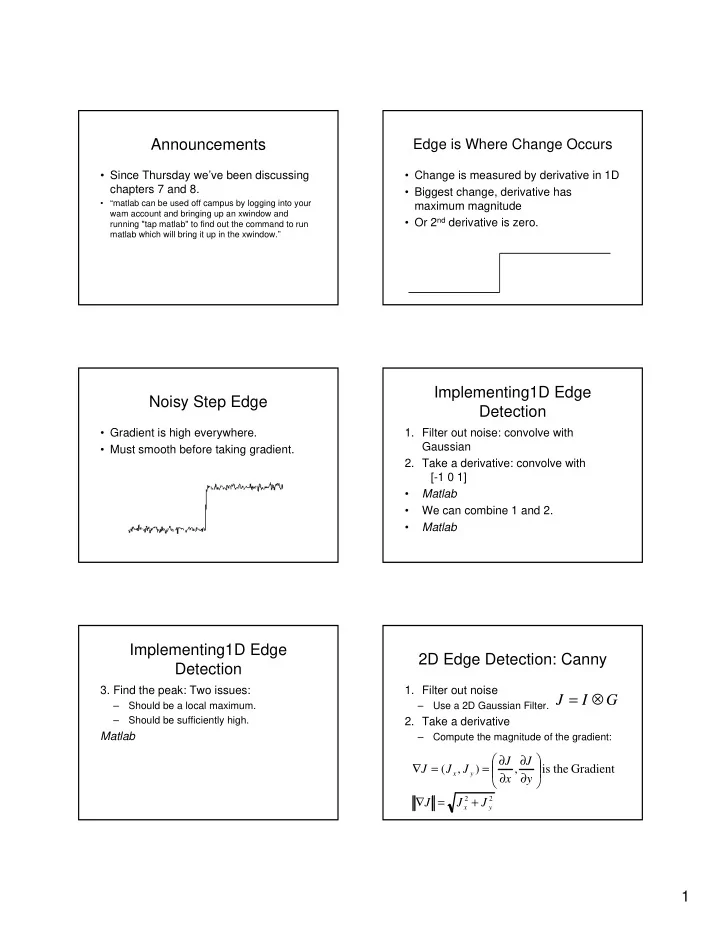
Noisy Step Edge
- Gradient is high everywhere.
- Must smooth before taking gradient.
Implementing1D Edge Detection
- 1. Filter out noise: convolve with
Gaussian
- 2. Take a derivative: convolve with
[-1 0 1]
- Matlab
- We can combine 1 and 2.
- Matlab
Implementing1D Edge Detection
- 3. Find the peak: Two issues:
– Should be a local maximum. – Should be sufficiently high.
Matlab
2D Edge Detection: Canny
- 1. Filter out noise
– Use a 2D Gaussian Filter.
- 2. Take a derivative
– Compute the magnitude of the gradient:
2 2
Gradient the is , ) , (
y x y x
J J J y J x J J J J + = ∇ ∂ ∂ ∂ ∂ = = ∇
G I J ⊗ =