
SLIDE 1
2D tensor network study of the
S=1 bilinear-biquadratic Heisenberg model
Philippe Corboz, Institute for Theoretical Physics, University of Amsterdam
- I. Niesen and P. Corboz, Phys. Rev. B 95, 180404 (2017)
- I. Niesen and P. Corboz, SciPost Phys. 3, 030 (2017)
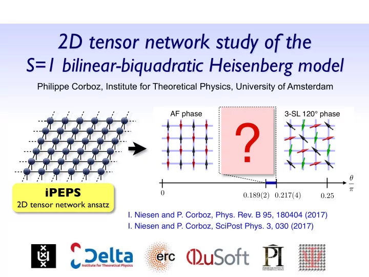
iPEPS
2D tensor network ansatz
θ π
0.25 AF phase Haldane phase 3-SL 120° phase 0.217(4) 0.189(2)