Introduction to Principles of integrity Information Visualization - - PowerPoint PPT Presentation

Introduction to Information Visualization

Kai Li Computer Science Department Princeton University

2

About This Talk

What is information visualization Principles of graphical excellence Principles of integrity Some visualization techniques References

E.R. Tufte, The Visual Display of Quantitative Information,

Graphics Press, 1983.

S.K. Card, J.D. Mackinlay, and B. Shneiderman, Information

Visualization: Using Vision to Think, Morgan Kaufmann Publishers, 1999.

3

What is Information Visualization?

Visualization:

“The action or fact of visualizing; the power or process of forming a mental picture or vision of something not actually present to the sight; a picture thus formed.” (Oxford English Dictionary)

Information visualization:

“Transformation of the symbolic into the geometric” (McCormick et al., 1987)

Information visualization:

“... finding the artificial memory that best supports our natural means of perception.'‘ (Bertin, 1983)

Information visualization:

“The use of computer-supported, interactive, visual representations of abstract data to simplify cognition.” (Card, Mackinlay, Shneiderman, 1999)

4

Power of Visualization

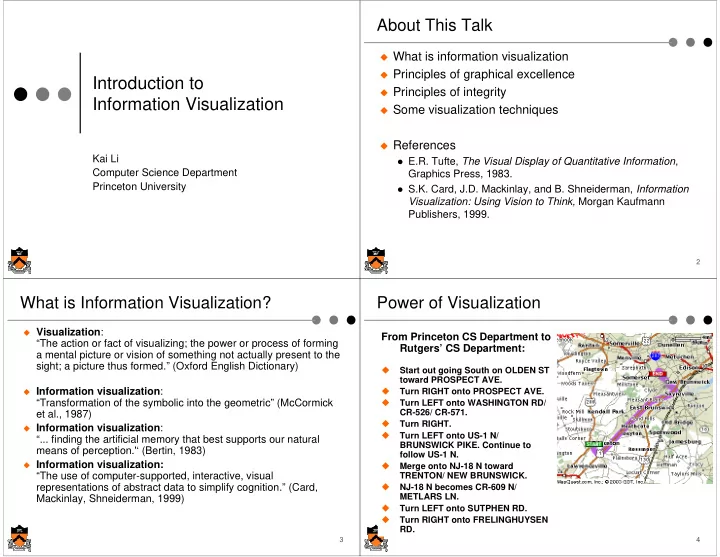
From Princeton CS Department to Rutgers’ CS Department:

• Start out going South on OLDEN ST

toward PROSPECT AVE.

• Turn RIGHT onto PROSPECT AVE.
• Turn LEFT onto WASHINGTON RD/

CR-526/ CR-571.

• Turn RIGHT.
• Turn LEFT onto US-1 N/

BRUNSWICK PIKE. Continue to follow US-1 N.

• Merge onto NJ-18 N toward

TRENTON/ NEW BRUNSWICK.

• NJ-18 N becomes CR-609 N/

METLARS LN.

• Turn LEFT onto SUTPHEN RD.
• Turn RIGHT onto FRELINGHUYSEN

RD.

5

Information Visualization

Problem

How to understand massive datasets?

Solution

Convert information into a graphical representation Take better advantage of human perceptual system

Issues

What is a good visualization? How to convert data?

6

Goals of Information Visualization

Make large datasets coherent Present huge amounts of information compactly Induce the viewer to think about the substance instead

• f methodology, design, technology, and so on

Encourage comparisons of different data Present information at several levels of detail, from

• verviews to fine structure

Tell stories about the data statistically

7

Statistical Visualization: Anscombe's Quartet

6.58 5.76 7.71 8.84 8.47 7.04 5.25 12.50 5.56 7.91 6.89 8.0 8.0 8.0 8.0 8.0 8.0 8.0 19.0 8.0 8.0 8.0 7.46 6.77 12.74 7.11 7.81 8.84 6.08 5.39 8.15 6.42 5.73 10.0 8.0 13.0 9.0 11.0 14.0 6.0 4.0 12.0 7.0 5.0 9.14 8.14 8.74 8.77 9.26 8.10 6.13 3.10 9.13 7.26 4.74 10.0 8.0 13.0 9.0 11.0 14.0 6.0 4.0 12.0 7.0 5.0 8.04 6.95 7.58 8.81 8.33 9.96 7.24 4.26 10.84 4.82 5.68 10.0 8.0 13.0 9.0 11.0 14.0 6.0 4.0 12.0 7.0 5.0 Y X Y X Y X Y X Data Set IV Data Set III Data Set II Data Set I

F.J. Anscombe, “Graphs in Statistical Analysis,” American Statistician, 27 (Feb 1973), pp17-21 8

Anscombe’s Scatter Plots

Positive linear Complex non-linear Linear w/ 1 outlier No variability except 1

9

Cholera Outbreak in London in 1854

The first death caused by cholera was

found in London in 1831.

The year 1853 saw outbreaks in Newcastle

and Gateshead as well as in London, where a total of 10,675 people died of the disease.

On August 31 of 1854, the outbreak of

cholera hit London Soho area: 127 people died in the next three days and 500 within 10 days.

What is causing a cholera epidemic in

London in 1854?

• Dr. John Snow suspected cholera was

transmitted by water, but could not prove it, then he used a map …

10

John Snow’s Map of Cholera Deaths

• Dr. John Snow plotted the location of

deaths from cholera in central London for Sept 1854. Deaths are marked by black dots. Water pumps are marked with red cycles.

11

Time Series: Wheat Prices, Wages and Kings and Queens (William Playfair, 1786)

Weekly wages of good mechanics Price of quarter

• f wheat

King or Queen

12

Today’s Time Series

13

Space & Time: Napoleon’s Army in Russia (Charles Joseph Minard, 1861)

“It may well be the best statistical graphic ever drawn.” Edward R. Tufte, 1983

14

A More Readable Version

15

Principles of Graphical Excellence

Graphical excellence is the well-designed presentation

• f interesting data – a matter of substance, of statistics,

and of design

Graphical excellence consists of complex ideas

communicated with clarity, precision, and efficiency

Graphical excellence is that which gives to the viewer

the greatest number of ideas in the shortest time with the least ink in the smallest space

Graphical excellence is nearly always multivariate Graphical excellence requires telling the truth about the

data E.R. Tufte 1983

16

Integrity Principle I

The representation of numbers, as physically measured on the

surface of the graphic itself, should be directly proportional to the numerical quantities represented

Measure of violation

Lie Factor (LF) = Size of effect shown in graphic Size of effect in data

Use logarithm of the Lie Factor to compare Overstating log LF > 0 Understating log LF < 0 Most distortions involve overstating; LF = 2-5 are common

17

Adapted from The New York Times, August 9, 1978, p. D-2

Fuel Economy Standards for Autos

Set by Congress and supplemented by the Transportation Department. In miles per gallon.

27 1/2 27 26

24

22

20

18

‘79 1978 ‘80 ‘81 ‘82 ‘83 ‘84 ‘85

Example Violated the Principle

18

Required Fuel Economy Standard: New Cars Built from 1978 to 1985

18 19 20 22 24 26 27 27.7 5 10 15 20 25 30 1978 1979 1980 1981 1982 1983 1984 1985 Miles per Gallon

Integrity Principle II

Clear, detailed, and

thorough labeling should be used to defeat graphical distortion and ambiguity

Write out explanations

• f the data on the

graphic itself

Label important events

in the data

19.1 mpg expected average for all cars

• n road, 1985

13.7 mpg average for all cars on road, 1978

19

Integrity Principle III

Show data variation, not design variation

20

Integrity Principle IV

In time-series displays of money, deflated and

standardized units of monetary measurement are always better than nominal units

21

Integrity Principle V

The number of

information-carrying (variable) dimensions depicted should not exceed the number of dimensions in the data

1958 - Eisenhower: $1.00 1963 - Kennedy: 94¢ 1968 - Johnson: 83¢

1973 - Nixon: 64¢

1978 - Carter: 44¢

Purchasing Power of the Diminishing Dollar

Source: Labor Department

Adapted from The Washington Post, October 25, 1978, p.1

Dollar value shrinks in

• ne dimension, but the

dollar sizes shrinks in 2 dimensions

22

1958 - Eisenhower: $1.00 1963 - Kennedy: 94¢ 1968 - Johnson: 83¢

1973 - Nixon: 64¢

1978 - Carter: 44¢

Purchasing Power of the Diminishing Dollar

Source: Labor Department

LF = 1

Now the area size of

the dollar shrinks at the same rate as the dollar value

23

Integrity Principle VI

Graphics must not quote data out of context 275 280 285 290 295 300 305 310 315 320 325 1955 1956 Traffic deaths

Connecticut traffic deaths, 1951-1959 225 235 245 255 265 275 285 295 305 315 325

1 9 5 1 1 9 5 2 1 9 5 3 1 9 5 4 1 9 5 5 1 9 5 6 1 9 5 7 1 9 5 8 1 9 5 9

Traffic deaths Before stricter enforcement After stricter enforcement

24

Data Ink Principle (Tufte, 1983)

Maximize the data-ink ratio Erase non-data-ink Erase redundant data-ink

Data-ink ratio Data-ink

=

Total ink used to print the graphic

HW 19% SW 15% Labor 41% Recover 13% Down 12% HW 19% SW 15% Labor 41% Recover 13% Down 12%

25

Example: Erase Redundant Data-Ink

19 15 43 13 12 16 46 15 11 18

20 40 60 HW SW Labor Recover Down 2000 1998

19 15 43 13 12

HW SW Labor Recover Down

18 16 46 15 11

1998 2000

26

Data Maps: Cancer Mortality by County

What do we learn from the maps? What’s wrong with the data maps?

27

Data Maps: Cancer Mortality by SEA

What do you think about these maps?

28

Data Maps: Cancer Mortality by SEA

What do we learn from these?

29

Data Maps: Breast Cancer by SEA

Big difference between male and female?

30

Data Maps: Breast Cancer by SEA Black vs. White Female

What can

31

What About This Familiar Data Map

32

Dimensions to Explore Data (Keim 97)

Geometric Icon-based Pixel-oriented Hierarchical Graph-based Mapping Projection Filtering Link&Brush Zooming

Distortion

Simple Complex

Data Visualization Interaction

33

Graphics primitives

The Key Is Visual Metaphor

Metaphor examples

Weather map Scatter plots

Reality Representation

• f reality (data)

Visual metaphor Picture(s) Viewer(s)

34

Basic Techniques

Scatter plot for point data

1-D: The data are points on a single axis 2-D: The pairs of values are points in a plane 3-D: Use color, brightness, and animation

Scalar Data

Line graph: Draw a line through a set of data points,

interpolating using straight line, spline curve, etc. (Lambert proposed drawing through middle of two points in 1765)

Multiple line graph: Display several plots on the same graph,

using line patterns (continuous, dot, dash), thickness, and color

Bar chart (pie charts similar): Depict values by lengths of bars Histogram: Data elements are placed into bins according to

value ranges, and draw bar charts on the numbers of elements of bins

35

Lifestreams

(Fertig, S., Freeman, E. and Gelernter, D. 1996)

View by time

36

2-D: Disk Areal Density vs. Time

37

Techniques for Multi-Dimensions

Place data using 2-D placements

Scatter-plot matrices, hyperslice, prosection Parallel coordinates Icon shapes Stick figures Pixel-oriented with tour, spiral, axes, circle segments Colors

Place data using 3-D projection, landscape

Isosurface Volume rendering Vector visualization

38

Isosurface Cells

For a given isovalue, only a

smaller portion of cells are isosurface cell.

For a volume with n x n x n

cells, the average number of the isosurface cells is n x n (ratio of surface v.s. volume)

The classical approach is

called “Marching cubes” which marches through all cells and figure out the isosurface n n n

39

Isosurface Extraction of Visible Woman

40

3-D Volume Rendering

41

Graphs

Types

Undirected graphs Directed graphs

CS Examples

Networks and wiring diagrams Finite state machines Dependencies Call graphs Pointers

42

Hierarchies

Techniques

Tree Tree-map: subdivide spaces for multiple dimensions Cone tree Info-cube

Examples

Organization Directory Abstraction

43

Early Treemap Applied to File System

44

www.smartmoney.com/marketmap

A TreeMap Application

45

Six Degrees of Mohamed Atta

(T.A. Stewart, December 2001 issue)

Valdis Krebs's examination of the interrelationships between the 19 hijackers in the 9/11 attack and the available connections by the authorities

46

Distortion

Problem

Small displays vs. large information space Tunnel vision Seeing the forest through the trees

Views

Local detail or focus Global context

Taxonomy

Multiple windows (overview and detail) Fisheye lens or selective distortion Pan and Zoom

47

Bifocal Display

Distortion at 1 or 2 dimensions with linear transformation Combination of detailed view and two distorted side views. 48

Perspective (Bifocal) Wall