
SLIDE 1
Introduction to Machine Learning Polynomial Regression Models
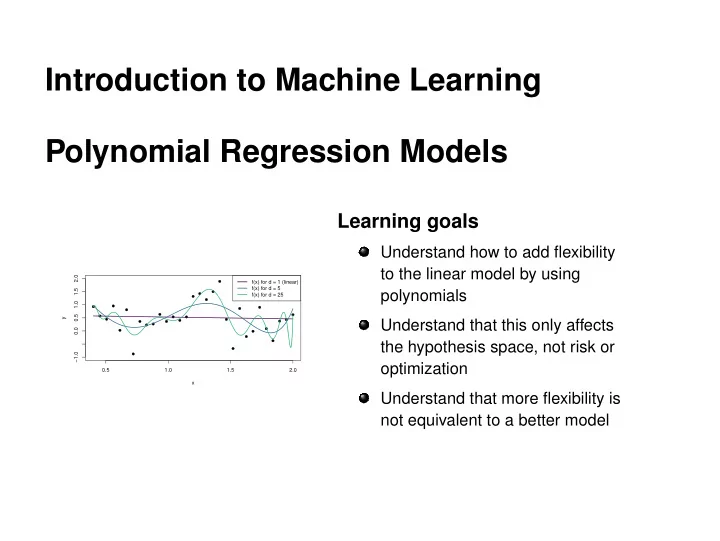
0.5 1.0 1.5 2.0 −1.0 0.0 0.5 1.0 1.5 2.0 x y f(x) for d = 1 (linear) f(x) for d = 5 f(x) for d = 25
Learning goals
Understand how to add flexibility to the linear model by using polynomials Understand that this only affects the hypothesis space, not risk or
- ptimization