Intro to Life Cycle Analysis Intro to Life Cycle Analysis Intro to - PowerPoint PPT Presentation

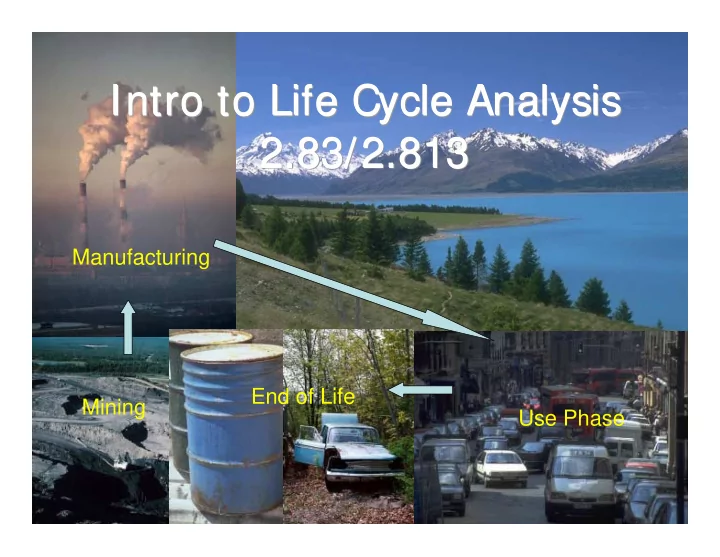
Intro to Life Cycle Analysis Intro to Life Cycle Analysis Intro to Life Cycle Analysis 2.83/2.813 2.83/2.813 2.83/2.813 Manufacturing End of Life Mining Use Phase

References 1. Allen and Shonnard, Ch 13 “ 1. “ Life Cycle Concepts Life Cycle Concepts … …” 1. 1. “ “ Life Cycle Concepts Life Cycle Concepts … … 2. 2. 2. 2. Hendrickson, Lave and Matthews, Chapters (1), 2, and 5, 6 & App. I 3. Leontief 3. 3. 3. Leontief Leontief Leontief, Input/Output Economics, pp19 – 24 (handout) 4. CMU I/O Website: 4. CMU I/O Website: Environmental Input-Output LCA: 4. CMU I/O Website: 4. CMU I/O Website: http://www.eiolca.net/ 5. 5. 5. 5. Sullivan et al Sullivan et al Sullivan et al Sullivan et al LCI of Family Sedan

Outline Outline Outline Outline 1. Streamlined Life Cycle Analysis 2. Process Level LCA 3. Input/Output LCA 4. Case Study: Automobiles 5. Other Examples (critique)

Life Cycle Analysis Life Cycle Analysis Life Cycle Analysis Life Cycle Analysis Mining Primary Mfg Distribution Use Disposition & & & & & & & & & & & & m m m m m m m m m m m m 0 0 0 0 0 0 8 8 8 8 8 8 & & & & & & m & m & m & m & m & m & m p o m p o m p o m p o m p o m p o p i p i p i p i p i p i k k k k k k k k k k k k Recycle, Remanufacture, Reuse

Life Cycle Inventory • LCA = LCI + Impact Analysis • i.e. counting the mercury emissions, and then accounting for their impact… • Issues: – transport, exposure, sensitivity – aggregating impacts – weighting impacts

Life Cycle Perspective Life Cycle Perspective Life Cycle Perspective Life Cycle Perspective • in theory boundaries start from earth as the source, and return to earth as the sink • evaluation is often focused on a product or service • tracking is of materials • time stands still

Streamlined Life Cycle Streamlined Life Cycle Streamlined Life Cycle Streamlined Life Cycle Assessment Assessment Assessment Assessment • qualitative assessment • value judgments by experts • for each stage of the life cycle • in broad categories of impact • “first cut” at the problem • See SLCA by T. Graedel 1998

Streamlined LCA INPUTS OUTPUTS air energy activity water mat’ls land Issues: 1. qualitative Vs quantitative 2. aggregation

Evaluation Matrix for SLCA, Evaluation Matrix for SLCA, M Evaluation Matrix for SLCA, Evaluation Matrix for SLCA, M M M ij ij ij ij Life Cycle Materials Energy Solid Liquid Gaseous Stages Choice Use Residues Residues Residues Extraction and 11 12 13 14 15 Refining Manufacturing 21 22 23 24 25 Product 31 32 33 34 35 Delivery Product Use 41 42 43 44 45 Refurbishment, 51 52 53 54 55 Recycling, Disposal Graedel

Scoring M 21 (mat’ls used in mfg) • M 21 = 0 when product mfg requires relatively large amounts of restricted mat’ls (limited supply, toxic, radioactive) and alternatives are available. • M 21 =4 when mat’ls used in mfg are completely closed loop and minimum inputs are required.

Automobile Example; Automobile Example; Automobile Example; Automobile Example; Manufacturing Ratings 0 Manufacturing Ratings 0 Manufacturing Ratings 0 Manufacturing Ratings 0- - -4 (best) - 4 (best) 4 (best) 4 (best) Element Designation Element Designation Element Value & Explanation: Element Value & Explanation: Element Value & Explanation: Element Value & Explanation: Element Designation Element Designation Element Value & Explanation: Element Value & Explanation: Element Value & Explanation: Element Value & Explanation: 1950s Auto 1950s 1950s 1950s Auto Auto Auto 1990s 1990s 1990s Auto 1990s Auto Auto Auto Matls. choice Chlorinated solvents, cyanide Good materials choices, except for lead solder waste 21 0 3 Energy use during manufacture is high Energy use during manufacture is fairly high Energy use 22 1 2 Solid residue Lots of metal scrap and packaging scrap produced Some metal scrap and packaging scrap produced 23 2 3 Liq. Residue Substantial liquid residues from cleaning and Some liquid residues from cleaning and painting 24 2 3 painting Gas residue Volatile hydrocarbons emitted from paint shop Small amounts of volatile hydrocarbons emitted 25 1 3 taken from Graedel 1998

Product Assessment Matrix for the Product Assessment Matrix for the Product Assessment Matrix for the Product Assessment Matrix for the Generic Generic Generic Generic 1950s 1950s Automobile [ 1950s 1950s Automobile [ Automobile [ Automobile [Graedel Graedel Graedel Graedel 1998] 1998] 1998] 1998] Environmental Stressor Life Cycle Stage Materials Energy Solid Liquid Gaseous Total Choice Use Residues Residues Residues Premanufacture 2 2 3 3 2 12/20 Product 0 1 2 2 1 6/20 Manufacture Product 3 2 3 4 2 14/20 Delivery Product Use 1 0 1 1 0 3/20 Refurbishment, 3 2 2 3 1 11/20 Recycling, Disposal Total 9/20 7/20 11/20 13/20 6/20 46/100

Product Assessment Matrix for the Product Assessment Matrix for the Product Assessment Matrix for the Product Assessment Matrix for the Generic Generic Generic Generic 1990s 1990s Automobile [ 1990s 1990s Automobile [ Automobile [ Automobile [Graedel Graedel Graedel Graedel 1998] 1998] 1998] 1998] Environmental Stressor Life Cycle Stage Materials Energy Solid Liquid Gaseous Total Choice Use Residues Residues Residues Premanufacture 3 3 3 3 3 15/20 Product 3 2 3 3 3 14/20 Manufacture Product 3 3 3 4 3 16/20 Delivery Product Use 1 2 2 3 2 10/20 Refurbishment, 3 2 3 3 2 13/20 Recycling, Disposal Total 13/20 12/20 14/20 16/20 13/20 68/100

Target plot Target plot of the estimated SLCA impacts for of the estimated SLCA impacts for Target plot Target plot of the estimated SLCA impacts for of the estimated SLCA impacts for generic automobiles for the 1950s and 1990s generic automobiles for the 1950s and 1990s generic automobiles for the 1950s and 1990s generic automobiles for the 1950s and 1990s Primary Mat’ls (1,1) End of Life 0 (5,5) (1,2) (5,4) (1,3) (5,3) 1 (1,4) (5,2) (1,5) 2 Mfg: Mat’l choices (5,1) (2,1) 3 (4,5) (2,2) 4 (4,4) (2,3) gas residues Mfg (4,3) (2,4) Use (4,2) (2,5) energy (4,1) (3,1) 1950s (3,5) (3,2) (3,4) (3,3) 1990s distribution [Graedel 1998]

Process Level LCA Process Level LCA Process Level LCA Process Level LCA 1 2 1 3 4 2 1 5 3 4 2 5 1 3 1 4 2 2 5 “Activity” 3 4 3 4 5 Issue: truncation error 5

Demand Vs Production Demand Vs Production Demand Vs Production Demand Vs Production 1 2 3 4 5 “Activity”

Demand Vs Production Demand Vs Production Demand Vs Production Demand Vs Production • f = “demand for 1” by 1 the “Activity” 2 • x = quantity of 1 3 produced to meet the 4 demand 5 “Activity” • x- α x = f • x = f/(1- α ) Because of interactions, “1” has to produce more “x” than “f” furthermore, 2, 3, 4, … have to produce to support “1”

Input/Output Analysis Input/Output Analysis Input/Output Analysis Input/Output Analysis 1 2 3 • f 1 = “demand for 1” by the “Activity 1” 4 5 6 • x i = quantity of “i” produced to meet 7 … the demand for “1” Physically we can think of subdividing the economy in sectors that interact with each other. The sectors include all activities so there are no truncation errors, however to be manageable we can only handle a few hundred sectors, therefore each sector will actually include a lot of different activities. “Aggregation errors”

Simplified input Simplified input Simplified input- Simplified input - -output table for a three - output table for a three output table for a three output table for a three- - - - sector economy sector economy sector economy sector economy Table 2.1 from Leontief, Oxford Press ’86 to Sector 1: Sector 2: Sector 3: Total : Agriculture Manufacture House- Output Holds From: Sector 1: 25 20 55 100 Agriculture bushels of wheat Sector 2: 14 6 30 50 yards Manufacture of cloth Sector 3: 80 180 40 300 man- Households years of labor

Rewrite as table in dollars Rewrite as table in dollars Rewrite as table in dollars Rewrite as table in dollars Ag Mfg. House Total (demand) (pro- duction) Ag x 11 x 12 f 1 x 1 Mfg x 21 x 22 f 2 x 2

In matrix form In matrix form In matrix form In matrix form (x 1 – x 11 ) – x 12 = f 1 -x 21 + (x 2 – x 22 ) = f 2 or using coefficients a ij = x ij /x j (1 – a 11 )x 1 – a 12 x 2 = f 1 -a 21 x 1 + (1 – a 22 )x 2 = f 2 or [I – a] {x} = {f}

[I – a] {x} = {f} 1 {f} a] - -1 - - 1 1 {x} = [I {x} = [I- {x} = [I {x} = [I - -a] - a] a] {f} {f} {f} {e} = [R]{x} 1 {f} a] - -1 - - 1 1 {e} = [R] [I {e} = [R] [I- {e} = [R] [I {e} = [R] [I - -a] - a] a] {f} {f} {f} where [R] is a matrix with diagonal elements (impact/dollar) and {e} = environmental impacts

CMU I/O website CMU I/O website CMU I/O website CMU I/O website http://www.eiolca.net/