
SLIDE 1
Intro to Life Cycle Analysis 2.83/2.813 Manufacturing End of Life - - PowerPoint PPT Presentation
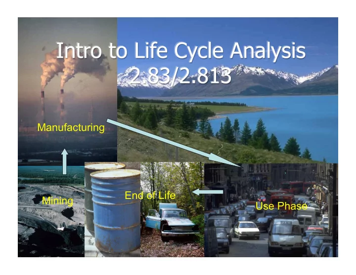
Intro to Life Cycle Analysis 2.83/2.813 Manufacturing End of Life Mining Use Phase Life Cycle Assessment LCA is a methodology to account for and assess the environmental impacts from all phases / stages of a product life cycle Mining
m
m
i p m
k
m m
m
i p m
k
m m
m
i p m
k
m m
m
i p m
k
m m
m
i p m
k
m m
m
i p m
k
m
LCA is a methodology to account for and assess the environmental impacts from all phases / stages of a product life cycle
Material mining and processing Product manufacturing Transportation Use End of Life
Energy Consumption:
Cooling? Distance dependent? Landfill?
Material mining and processing Product manufacturing Transportation Use End of Life
Six Products, Six Carbon Footprints, WSJ, 2009
Product Descending Order of Energy Consumption Car 4>2 >1 >5 >3 Shoes 1>3 >2 >5 >4 Laundry Detergent 4>1 >2 >3 >5 Fleece Jacket 1>2 >4 >3 >5 Beer 1>2 >4 >3 >5 Milk 3>2 >4 >1 >5
Measuring the Footprints
Greenhouse-gas emissions associated with six common products*
Retail (mostly refrigerating the beer at the store) Glass for the beer bottles Barley Malt Distribution (trucking beer from brewery to distributor and store) Use (keeping the beer cold in a consumer’s refrigerator) Brewing operations (natural gas used at brewery) 3.9% Paper (beer-bottle labels and six-pack box) 2.3% Added carbon dioxide (used to help carbonate the beer) 2.3% Other Electricity used in shoe assembly Producing the raw materials Making the materials for the car (steel, plastic, etc.) Assembling the car Producing the fuel and transporting it to the gas station Fuel use in the car Vehicle maintenance 4.7% Disposing of the car Making the liquid detergent Transporting the detergent from the factory to the store 0.2% Energy use in store 1% 73% Disposal of the package Producing the polyester Making the fabric and assembling the jacket Design and marketing 0.5% Growing the feed and hay bedding for the cows Transporting the feed to the dairy farm Cows’ enteric fermentation Fuel and electricity use on dairy farm Transporting the raw milk to the processing plant 2% Fuel and electricity use at the processing plant Packaging for the milk Storing the packaged milk at the processing plant and transporting it to a distribution center Other 3% 6.6% 28.1% 21.6% 12.6% 6% 8.4% 8.2% 52.7% 15.8% 12.9% 8.3% 12% 7% 6% 5% 8% 6% 28% 23% 28.9% 70.8% 7% 93% 9% 17%
†Includes emissions from producing the oil that's used to make the polyester through the jacket’s arrival at Patagonia’s distribution center in Reno, Nev. Doesn’t include transportation from the distribution center to retail stores, which Patagonia says is negligible. ††Data for a half-gallon of Aurora organic milk; number for other milks may vary *Footprints are expressed in carbon-dioxide-equivalent pounds. Percentages may not total 100% due to rounding. Note: Based on a 1.5-liter bottle (about 1.5 quarts), 20 loads per bottle and 9.9 pounds of laundry per load. Note: Assumes a 2007 Prius, driven 126,000 miles over its life and getting 42 miles per gallon.
Use (mostly energy to power the washing machine and heat the water)
Sources: Toyota; Kreider & Associates; Timberland; Tesco; Patagonia; New Belgium Brewing Co.; Aurora Organic Dairy; University of Michigan’s Center for Sustainable Systems
5.7%
CAR Toyota Prius
TOTAL FOOTPRINT: 97,000 pounds
PAIR OF HIKING BOOTS Timberland Winter Park Slip On Boots
TOTAL FOOTPRINT: 121 pounds
LAUNDRY DETERGENT Tesco Non-Biological Liquid Wash
TOTAL FOOTPRINT: 31 pounds
SIX-PACK OF BEER Fat Tire Amber Ale
TOTAL FOOTPRINT: 7 pounds
FLEECE JACKET Patagonia Talus jacket
TOTAL FOOTPRINT: 66 pounds†
HALF-GALLON OF MILK Aurora Organic Dairy
TOTAL FOOTPRINT: 7.2 pounds††
Cows’ manure
Six Products, Six Carbon Footprints, WSJ, 2009
ISO 14044 and other 14000
energy mat’ls land water air
Product
energy mat’ls land water air
Product
Life Cycle Stages Materials Choice Energy Use Solid Residues Liquid Residues Gaseous Residues Extraction and Refining 11 12 13 14 15 Manufacturing 21 22 23 24 25 Product Delivery 31 32 33 34 35 Product Use 41 42 43 44 45 Refurbishment, Recycling, Disposal 51 52 53 54 55
Graedel
Element Designation Element Value & Explanation: 1950s Auto Element Value & Explanation: 1990s Auto
21
Chlorinated solvents, cyanide
3
Good materials choices, except for lead solder waste
Energy use 22
1
Energy use during manufacture is high
2
Energy use during manufacture is fairly high
Solid residue 23
2
Lots of metal scrap and packaging scrap produced 3 Some metal scrap and packaging scrap produced
24
2
Substantial liquid residues from cleaning and painting
3
Some liquid residues from cleaning and painting
Gas residue 25
1
Volatile hydrocarbons emitted from paint shop
3
Small amounts of volatile hydrocarbons emitted
taken from Graedel 1998
Environmental Stressor
Life Cycle Stage Materials Choice Energy Use Solid Residues Liquid Residues Gaseous Residues Total Premanufacture 2 2 3 3 2 12/20 Product Manufacture 1 2 2 1 6/20 Product Delivery 3 2 3 4 2 14/20 Product Use 1 1 1 3/20 Refurbishment, Recycling, Disposal 3 2 2 3 1 11/20
Total 9/20 7/20 11/20 13/20 6/20 46/100
Environmental Stressor
Life Cycle Stage Materials Choice Energy Use Solid Residues Liquid Residues Gaseous Residues Total Premanufacture 3 3 3 3 3 15/20 Product Manufacture 3 2 3 3 3 14/20 Product Delivery 3 3 3 4 3 16/20 Product Use 1 2 2 3 2 10/20 Refurbishment, Recycling, Disposal 3 2 3 3 2 13/20
Total 13/20 12/20 14/20 16/20 13/20 68/100
4 3 2 1 (1,1) (1,2) (1,3) (1,4) (1,5) (2,1) (2,2) (2,3) (2,4) (2,5) (3,1) (3,2) (3,3) (3,4) (3,5) (4,1) (4,2) (4,3) (4,4) (4,5) (5,1) (5,2) (5,3) (5,4) (5,5)
1950s 1990s
[Graedel 1998] Mfg: Mat’l choices Use Primary Mat’ls Mfg distribution End of Life energy gas residues
TABLE 1. EMPERICAL MANUFACTURING ENERGY STUDIES
Manufacturing Process Source
Coventional Manufacturing Machining 5.3
Milling 1.3
Grinding [5] Iron Casting 19
[3] Sand casting 11.6
[6] die casting [7] Forging [8] Finish Machining [9] Advanced Manufacturing Waterjet (Nylon) 150
Waterjet (Steel) 167
Waterjet (Al) 195
Energy Requirement Range (MJ/kg processed)
[10] [4] 24 16.3 8.8 14.9
[ 1 ]
Table 1: N. Duque Ciceri, T. G. Gutowski, M. Garetti, 2010, and Table 2: Young S. Song, Jae R. Youn, Timothy G. Gutowski,
Manufacturing methods Energy intensity (MJ/kg) Autoclave molding 21.9a Spray up 14.9b Resin transfer molding (RTM) 12.8b Vacuum assisted resin infusion (VARI) 10.2b Cold press 11.8b Preform matched die 10.1b Sheet molding compound (SMC) 3.5b Filament winding 2.7b Pultrusion 3.1b Prepreg production 40.0b Injection molding (hydraulic) 19.0c Glass fabric manufacturing 2.6d Iron casting (Cupola) 13.6e
Table 2
See Ashby Ch. 7 for basic assumptions and Ch 9 for a comparison between various beverage container options
“Activity” 1 2 3 4 5 1 2 3 4 5 1 2 3 4 5 1 2 3 4 5 1 2 3 4 5
Sullivan et al SAE 1998
Plastics 9.3% Ferrous 64% Non- ferrous 9% Fluids 4.8% Other 13% Total 100%
Total Energy Use by Lifecycle Stage
100 200 300 400 500 600 700 800 900 Material Production Manufacturing Use Maintenance and Repair End of Life
Lifecycle Stage Total Energy Energy Use Use Per Per Car Car (GJ)
Sullivan 1998 Total Energy 973 GJ/car
Table 1 Eco-Audit Audit for
Sull lliv ivan’s n’s Au Auto tomobi
e (Pr Primarily y using using ene energy gy values values fr from Smil) il) Bill ll of Ma Materia ials (BOM) Mass ass (kg) g) MJ/ J/kg Energy gy (MJ) J) Plastics (PUR, PVC, Nylon, ABS…) 143kg 100 MJ/kg 14,300 Non-Ferrous Alu 93kg 200 18,600 Cu 18 100 1,800 Brass (Copper ~ 65%, zinc ~ 35%) 8.5 90 765 Lead 13 50 650 Other (Zn, Cr…) 5.5 30 165 Iron 156.5 kg 25 3,913 Steel 828.5 kg 50 41,425 Fluids (gasoline, oil,….) 74 10 740 Rubber (not tire) 60 100 6,000 Glass 42 20 820 Tires 45 100 4,500 Other (textiles, carpet…) 45 20 900 TOTAL TOTAL 94,578 94,578
Sullivan result: 94,460!
Tables from Smil, 2008
“Activity” 1 2 3 4 5 1 2 3 4 5 1 2 3 4 5 1 2 3 4 5 1 2 3 4 5
“Activity” 1 2 3 4 5
Each sector may have to produce “extra” to satisfy not only the identified “activity” but also to provide for all of the inputs
“Activity” 1 2 3 4 5
Table 2.1 from Leontief, Oxford Press ’86 From: to : Sector 1: Agriculture Sector 2: Manufacture Sector 3: House- Holds Total Output Sector 1: Agriculture
bushels of wheat Sector 2: Manufacture
Sector 3: Households
years of labor
Physical Units Dollars
see Ch 6 of HLM
Ref HLM Ch 6
Su Summ mmary f for Dif Different ent M Mode
ng App Approaches
Late 1990’s – early 2000’s family auto (~1500 kg) Mode
Mate ateria ials (GJ) (GJ) Mfg (GJ (GJ) ) Tota Total (GJ) (GJ) Sullivan 94.5 39 133.5 HLM (Ch 6 see text p 73) 138 EIOLCA 1997 ($16,009 –HLM deflator, producer price) 121 EIOLCA 1997 ($15,276 –cpi deflator, producer price) 116 EIOLCA 2002 ($17,126 producer price) 143 Eco-Audit (above) 94.6 30.6 (est 20MJ/kg) 125 Mean Mean Value Value (n=6) (n=6) 129.4 129.4 Standard Deviation 9.5 9.5 (a (abo bout ut 7% 7%)
Weber, C.L., The Importance of Carbon Footprint Estimation Boundaries Environ. Sci. Technol. 2008, vol. 42, pp 5839 – 5842.
1 2 3 4 5
Consultants
International/University of Stuttgart (IKP)/PE Product Engineering
Environmental Product Development
Ecobalance, Inc.
Umweltinformatik
The Focus of this presentation is on Navigation. Please refer to the “Wood Example” tutorial online for instructions on creating a full LCA. 1) Open Simapro 2) This is the first screen you see: Click here to open a library and browse.
Imagine we are interested in the LCI of a cardboard box
Click to obtain LCI Double Click to
LCI Click to obtain tree diagram of LCI
No Substance Compartment Unit Total Production cardboard box I Paper wood-free C B250 1 Additives Raw kg 0.007 0.007 x 2 Artificial fertilizer Raw kg 0.0000473 x 0.0000473 3 Bauxite, in ground Raw kg 0.00000343 x 0.000000879 4 Biomass Raw kg 0.000629 x 0.000629 5 Clay, unspecified, in ground Raw kg 0.013 x 0.013 6 Coal, 18 MJ per kg, in ground Raw kg 0.0146 x 0.0021 7 Coal, brown, 8 MJ per kg, in ground Raw kg 0.0112 x 0.00135 8 Complexing agent Raw kg 0.00000417 x 0.00000417 9 Defoamer Raw kg 0.0000158 x 0.0000158 10 Energy, potential, stock, in barrage water Raw MJ 0.688 x 0.0567 11 Gas, natural, 35 MJ per m3, in ground Raw m3 0.00247 x x 12 Gas, natural, 36.6 MJ per m3, in groundRaw m3 0.0154 x 0.0106 13 Gas, natural, feedstock, 35 MJ per m3, in ground Raw m3 0.0051 x x 14 Glue Raw kg 0.0052 0.0052 x 15 Ink Raw kg 0.0183 0.0183 x 16 Iron ore, in ground Raw kg 0.000002 x 0.000000302 17 Limestone, in ground Raw kg 0.0232 x 0.0232 18 Magnesium sulfate Raw kg 0.0000251 x 0.0000251 19 Manure Raw kg 0.00506 x 0.00506 20 Oil Raw kg 0.0002 0.0002 x 21 Oil, crude, 42.6 MJ per kg, in ground Raw kg 0.0202 x 0.00254 22 Oil, crude, feedstock, 41 MJ per kg, in ground Raw kg 0.00561 x 0.0011 23 Pesticides Raw kg 0.00000407 x 0.00000407 24 Potatoes Raw kg 0.00105 x 0.00105 25 Sand and clay, unspecified, in ground Raw kg 0.00000017 x x 26 Sand, unspecified, in ground Raw kg 0.000000135 x 0.000000135 27 Sodium chloride, in ground Raw kg 0.000817 x 0.000749
Weighting of the damage categories by the panel • http://www.pre.nl/default.htm
Ashby 2009 McMillan & Keoleian 2009
Aluminum from bauxite 190 - 230 MJ/kg
200 - 240 MJ/kg
115 MJ/kg
84 MJ/kg
Ashby 2009: 11 - 14 kgCO2/kg Also see debate on CNW’s report
Comparison of PRODUCTS' MATERIAL EMBOIDED ENERGY DATA: Calculated with BOM tool vs. LCIs Published
Natalia Duque Ciceri, 2009