Interphase Mass Transfer see Handout At equilibrium a species - - PowerPoint PPT Presentation

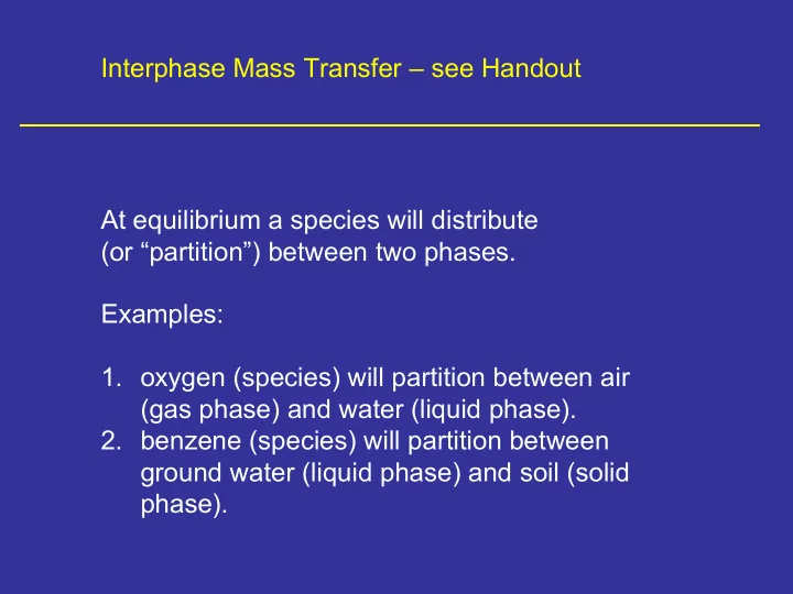
Examples: 1.

• xygen (species) will partition between air

(gas phase) and water (liquid phase). 2. benzene (species) will partition between ground water (liquid phase) and soil (solid phase). Interphase Mass Transfer – see Handout At equilibrium a species will distribute (or “partition”) between two phases.

Equilibria are quantified by specific “distribution laws”. An example of a distribution law is given by Henry’s Law, which is used to calculate the liquid phase concentration of a gas (i.e., gas solubility): pO2 = xO2 HO2

see Question 1 (page 2) for an example calculation.

pO2 ≈ cO2 HO2 MH2O /(cH2O MO2 ) If liquid is water, and gas is rather insoluble in liquid (like oxygen):

Distance Concentration of oxygen pi

O2

ci

O2

Interface Gas Phase Liquid Phase

= cl

O2 (8.5 mg/L)

= pg

O2 (160 mm Hg)

At equilibrium:

Consider now the physical situation: Two phases are suddenly brought into contact in which concentrations of the species are not in equilibrium. Let us contemplate this situation using the specific example of a gas containing oxygen at a concentration of pg

O2

and a liquid containing

• xygen at a concentration of cl

O2

, such that the species oxygen will be transferring from the gas to the liquid.

Not at equilibrium:

Distance Concentration of oxygen

Interface Gas Phase Liquid Phase

cl

O2

pg

O2

What happens? Two-resistance theory proposes that rate of diffusion across a microscopic interface is instantaneous, and that therefore equilibrium at the interface “locally” will be achieved immediately (“local equilibrium”). However, in either bulk solution (distant from the interface) the concentration will not have changed. Thus, a concentration gradient will develop in each phase.

Moving towards equilibrium:

Distance Concentration of oxygen pi

O2

ci

O2

Interface Gas Phase Liquid Phase

cl

O2

pg

O2

Direction of Flux δG δL

How do we predict the flux? Flux

∝

Concentration Gradient Flux (Phase I) = Flux (Phase II) = ΦO2 Flux (Gas Phase) ∝ (pg

O2

– pi

O2

) Flux (Liquid Phase) ∝ (ci

O2

– cl

O2

) Flux

∝

Concentration Difference However, we don’t have values for film thicknesses (δG , δL ) So, we can write a proportionality in either phase: Note also that if system is at steady-state:

For each phase we will define a proportionality constant called a mass transfer coefficient such that: (pg

O2

– pi

O2

) is the “gas phase driving force” for mass transfer (ci

O2

– cl

O2

) is the “liquid phase driving force” for mass transfer ΦO2 = kG (pg

O2

– pi

O2

) ΦO2 = kL (ci

O2

– cl

O2

) I.3 I.4

Good News:

1.

kL depends only

• n liquid phase, while kG

depends

• nly
• n gas phase.

2.

Knowing properties of that one phase (e.g., viscosity, density, velocity) allows us to calculate kL , kG empirically. (Really) Bad News:

1.

We don’t know values for interface concentrations. ΦO2 = kG (pg

O2

– pi

O2

) ΦO2 = kL (ci

O2

– cl

O2

)

We would really like to have a mass transfer coefficient which is related to the total, overall driving force… The problem with (pg

O2

– cl

O2

) is that these two concentrations are in different phases (one in terms of pressure and the other in terms of liquid concentration). We cannot compare the two concentrations directly. We’d like to have something like ΦO2

∝

(pg

O2

– cl

O2

)!

However, we can relate the gas phase concentration (pg

O2

) to the liquid phase concentration that would theoretically be in equilbrium with that concentration (c*O2 ). So, instead of the overall driving force being (pg

O2

– cl

O2

), it is (c*O2 – cl

O2

). We define an overall mass transfer coefficient KL as: Remember, c*O2 is in equilibrium with pg

O2

. If the equilibrium relationship is linear, then ΦO2 = KL (c*O2 – cl

O2

) I.6 pg

O2

= mO2 c*O2 I.9

Similarly, we can relate the liquid phase concentration (cl

O2

) to the gas phase concentration that would theorectically be in equilbrium with that concentration (p*O2 ). In this case, we define an overall mass transfer coefficient KG as: ΦO2 = KG (pg

O2

– p*O2 ) I.5 In this case, p*O2 is in equilibrium with cl

O2

. If the equilibrium relationship is linear, then p*O2 = mO2 cl

O2

I.8

Good News:

1.

The concentrations at the interface do not appear in the equations. Bad News:

1.

KG and KL depend on properties of both phases (strictly, but we often make a simplification!) ΦO2 = KG (pg

O2

– p*O2 ) ΦO2 = KL (c*O2 – cl

O2

)

KG –

• verall mass transfer coefficient in terms of gas phase

driving force KL –

• verall mass transfer coefficient in terms of liquid phase

driving force

Derive relationship between KL and kG , kL : c*O2 – cl

O2

= (c*O2 – ci

O2

) + (ci

O2

– cl

O2

) Divide each term by ΦO2 c*O2 – cl

O2

(c*O2 – ci

O2

) (ci

O2

– cl

O2

) = ΦO2 ΦO2 ΦO2 + c*O2 – cl

O2

(pg

O2

– pi

O2

) (ci

O2

– cl

O2

) = ΦO2 ΦO2 mΦO2 + Note that pg

O2

= mO2 c*O2 and pi

O2

= mO2 ci

O2

From the definitions of mass transfer coefficients… c*O2 – cl

O2

(pg

O2

– pi

O2

) (ci

O2

– cl

O2

) = ΦO2 ΦO2 mΦO2 + Similarly… 1 = kL KL mkG + 1 1 1 = kL KG kG + 1 m

Consider two extreme cases: 1 = kL KG kG + 1 m 1) gas is very soluble in liquid (NH3 in H2 O) m is very small KG ≈ kG We can use gas phase properties to calculate an overall mass transfer coefficient

2) gas is very insoluble in liquid (O2 in H2 O) m is very large KL ≈ kL We can use liquid phase properties to calculate an overall mass transfer coefficient 1 = kL KL mkG + 1 1

ΦNH3 = KG (pg

NH3

– p*NH3 ) ΦO2 = KL (c*O2 – cl

O2

) ΦNH3 = kG (pg

NH3

– p*NH3 ) ΦO2 = kL (c*O2 – cl

O2

) can be “simplified” to yield: Two mass transfer expressions ΦO2 = kG (pg

O2

– p*O2 ) Note, we can’t write:

(Only) Good News:

1.

kL depends only

• n liquid phase, while kG

depends

• nly
• n gas phase.

2.

Knowing properties of that one phase (e.g., viscosity, density, velocity) allows us to calculate kL , kG empirically.

3.

We can calculate all the concentrations, in particular p*O2 and c*O2 . ΦNH3 = kG (pg

NH3

– p*NH3 ) ΦO2 = kL (c*O2 – cl

O2

)