? ( interest - - PowerPoint PPT Presentation

interest point
SMART_READER_LITE
LIVE PREVIEW

? ( interest - - PowerPoint PPT Presentation

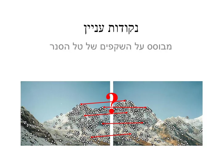
? ( interest point ) detection ( interest point


slide-1
SLIDE 1

ןיינע תודוקנ

לט לש םיפקשה לע ססובמרנסה

?

slide-2
SLIDE 2

םויהל םיאשונה

  • הנומתב תוניינעמ תודוקנ רותיא(

interest point detection )

  • הנומתב תודוקנ רואת(

interest point description )

  • תודוקנ ירואת ןיב תומאתה תאיצמ(

interest point matching )

slide-3
SLIDE 3

תורוקמ

  • קרפ4 דומילה רפסב
  • סרוק לש דומילה רפס"הנומת דוביע "

Gonzalez & Woods, “Digital Image Processing, 3rd edition”

slide-4
SLIDE 4

ןיינעמ עדימ אצמנ הנומתב הפיא?

slide-5
SLIDE 5

Image matching

by Diva Sian by swashford

slide-6
SLIDE 6

Harder case

by Diva Sian by scgbt

slide-7
SLIDE 7

Harder still?

NASA Mars Rover images

slide-8
SLIDE 8

NASA Mars Rover images with SIFT feature matches Figure by Noah Snavely

Answer below (look for tiny colored squares…)

slide-9
SLIDE 9

Local features and alignment

[Darya Frolova and Denis Simakov]

  • We need to match (align) images
  • Global methods sensitive to occlusion, lighting, parallax
  • effects. So look for local features that match well.
  • How would you do it by eye?
slide-10
SLIDE 10

Local features and alignment

  • Detect feature points in both images

[Darya Frolova and Denis Simakov]

slide-11
SLIDE 11

Local features and alignment

  • Detect feature points in both images
  • Find corresponding pairs

[Darya Frolova and Denis Simakov]

slide-12
SLIDE 12

Local features and alignment

  • Detect feature points in both images
  • Find corresponding pairs
  • Use these pairs to align images

[Darya Frolova and Denis Simakov]

slide-13
SLIDE 13

Local features and alignment

  • Problem 1:

– Detect the same point independently in both images

no chance to match!

We need a repeatable detector

[Darya Frolova and Denis Simakov]

slide-14
SLIDE 14

Local features and alignment

  • Problem 2:

– For each point correctly recognize the corresponding one

?

We need an invariant and distinctive descriptor

[Darya Frolova and Denis Simakov]

slide-15
SLIDE 15

Geometric transformations

slide-16
SLIDE 16

Photometric transformations

Figure from T. Tuytelaars ECCV 2006 tutorial

slide-17
SLIDE 17

And other nuisances…

  • Noise
  • Blur
  • Compression artifacts
slide-18
SLIDE 18

Invariant local features

Subset of local feature types designed to be invariant to common geometric and photometric transformations. Basic steps: 1) Detect distinctive interest points 2) Extract invariant descriptors 3) Match them!

Figure: David Lowe

slide-19
SLIDE 19

Main questions

  • Where will the interest points come from?

– What are salient features that we’ll detect in multiple views?

  • How to describe a local region?
  • How to establish correspondences, i.e.,

compute matches?

slide-20
SLIDE 20
slide-21
SLIDE 21

Finding Corners

  • Corners are repeatable and distinctive
  • Key property: in the region around a corner,

image gradient has two or more dominant directions

C.Harris and M.Stephens. "A Combined Corner and Edge Detector.“ Proceedings of the 4th Alvey Vision Conference: 1988, pages 147--151.

Source: Lana Lazebnik

slide-22
SLIDE 22

סירה לש תוניפה רתאמ: הניפ יהמ?

  • תישאר , תרוכזת– טנאידרגה

x y

f f f I I x y                 

Based on slides by Robert Collins, Pen State, 04

slide-23
SLIDE 23

סירה לש תוניפה רתאמ: הניפ יהמ?

  • תישאר , תרוכזת– טנאידרגה

x y

f f f I I x y                 

Based on slides by Robert Collins, Pen State, 04

slide-24
SLIDE 24

סירה לש תוניפה רתאמ: הניפ יהמ?

  • תישאר , תרוכזת– טנאידרגה

x y

f f f I I x y                 

Based on slides by Robert Collins, Pen State, 04

slide-25
SLIDE 25

רוזיפ ןויפאםיטנאידרגה

  • הספילא תודוקנל םיאתנ( תוגלפתהתינאיסואג )תישארב הזכרמש
  • איה הניפ" :לודג לוגיעל המודה הספילא " בחרמבםיטנאידרגה
  • איה הניפ : תוגלפתהתינאיסואג בחרמב םיריצ ינשב ההובג תונוש םע

םיטנאידרגה

Based on slides by Robert Collins, Pen State, 04

slide-26
SLIDE 26

תורבתסה תצק

  • תרוזפת תצירטמ(

scatter matrix / ) תצירטמ תפתושמ תונוש( covariance matrix )

  • יהת:
  • ידי לע תרדגומ תפתושמה תונושה תצירטמ:
  • M

הספילאה תא הרידגמ : םה םיימצעה היכרע הספילאה יריצ יכרא!

1 12 x xn y yn n

I I A I I

      

2

n w 

2 2 2 2 x x y T x y y

I I I M AA I I I

         

   

!תישארה איה תיתימאה תוגלפתהה עצוממ יכ החנהה תחת

slide-27
SLIDE 27

הרבגלא תצק :םיימצע םירוטקוו םיכרע

1

x

2

x

1

2

slide-28
SLIDE 28

הרבגלא תצק :םיימצע םירוטקוו םיכרע

  • The eigenvectors of a matrix A are the vectors x that satisfy:
  • The scalar  is the eigenvalue corresponding to x
  • The eigenvalues are found by solving:

– In our case, A = M is a 2x2 matrix, so we have – The solution:

  • Once you know , you find x by solving

11 12 21 22

det M M M M           

   

2 11 22 12 21 11 22

1 4 2 M M M M M M            

11 12 21 22

M M x M M y                 

Based on slides by Neel Joshi, UW, 10

slide-29
SLIDE 29

ונניינעל הרזח

  • הניפ ונל שי יכ עדנ ךיא זא ? היכרע ינשב ןנובתנ

לש םיימצעה M

1 2 “Corner” 1 and 2 are large,

1 ~ 2

1 and 2 are small; “Edge” 1 >> 2 “Edge” 2 >> 1 “Flat” region

slide-30
SLIDE 30

סיראה לש תוניפה ההזמ

  • וא ,בושיחל ליעי רתוי:

“Corner” R > 0 “Edge” R < 0 “Edge” R < 0 “Flat” region |R| small

2 2 1 2 1 2

) ( ) ( trace ) det(            M M R

α: constant (0.04 to 0.06)

slide-31
SLIDE 31

Harris Corner Detector

  • Algorithm steps:

– Compute M matrix within all image windows to get their R scores – Find points with large corner response (R > threshold) – Take the points of local maxima of R

slide-32
SLIDE 32

Harris Detector: Workflow

slide-33
SLIDE 33

Harris Detector: Workflow

Compute corner response R

slide-34
SLIDE 34

Harris Detector: Workflow

Find points with large corner response: R>threshold

slide-35
SLIDE 35

Harris Detector: Workflow

Take only the points of local maxima of R

slide-36
SLIDE 36

Harris Detector: Workflow

slide-37
SLIDE 37

Harris Detector: Properties

  • Rotation invariance

Ellipse rotates but its shape (i.e. eigenvalues) remains the same Corner response R is invariant to image rotation

slide-38
SLIDE 38

Harris Detector: Properties

  • Not invariant to image scale

All points will be classified as edges

Corner !

slide-39
SLIDE 39
  • How can we detect scale invariant interest

points?

slide-40
SLIDE 40

Option1: Exhaustive search

  • Multi-scale approach

Slide from T. Tuytelaars ECCV 2006 tutorial

slide-41
SLIDE 41

Option1: Exhaustive search

  • Multi-scale approach
slide-42
SLIDE 42

Option1: Exhaustive search

  • Multi-scale approach

Too Time consuming!

slide-43
SLIDE 43

Scale Invariant Detection

  • Consider regions (e.g. circles) of different sizes

around a point

  • Regions of corresponding sizes will look the same

in both images

slide-44
SLIDE 44

Scale Invariant Detection

  • The problem: how do we choose corresponding

circles independently in each image?

slide-45
SLIDE 45

Option 2: Invariance

  • Extract patch from each image individually

But how?

slide-46
SLIDE 46

Automatic scale selection

  • Solution:

– Design a function on the region, which is “scale invariant” (the same for corresponding regions, even if they are at different scales)

Example: average intensity. For corresponding regions (even of different sizes) it will be the same. scale = 1/2

– For a point in one image, we can consider it as a function of region size (patch width) f

region size Image 1

f

region size Image 2

slide-47
SLIDE 47

Automatic scale selection

  • Common approach:

scale = 1/2

f

region size Image 1

f

region size Image 2

Take a local maximum of this function Observation: region size, for which the maximum is achieved, should be invariant to image scale. s1 s2

Important: this scale invariant region size is found in each image independently!

slide-48
SLIDE 48
  • K. Grauman, B. Leibe

Automatic Scale Selection

  • Function responses for increasing scale (scale signature)

48

  • K. Grauman, B. Leibe

)) , ( (

1

 x I f

m

i i 

)) , ( (

1

 x I f

m

i i

slide-49
SLIDE 49
  • K. Grauman, B. Leibe

Automatic Scale Selection

49

  • K. Grauman, B. Leibe

)) , ( (

1

 x I f

m

i i 

)) , ( (

1

 x I f

m

i i

  • Function responses for increasing scale (scale signature)
slide-50
SLIDE 50
  • K. Grauman, B. Leibe

Automatic Scale Selection

50

  • K. Grauman, B. Leibe

)) , ( (

1

 x I f

m

i i 

)) , ( (

1

 x I f

m

i i

  • Function responses for increasing scale (scale signature)
slide-51
SLIDE 51
  • K. Grauman, B. Leibe

Automatic Scale Selection

51

  • K. Grauman, B. Leibe

)) , ( (

1

 x I f

m

i i 

)) , ( (

1

 x I f

m

i i

  • Function responses for increasing scale (scale signature)
slide-52
SLIDE 52
  • K. Grauman, B. Leibe

Automatic Scale Selection

52

  • K. Grauman, B. Leibe

)) , ( (

1

 x I f

m

i i 

)) , ( (

1

 x I f

m

i i

  • Function responses for increasing scale (scale signature)
slide-53
SLIDE 53
  • K. Grauman, B. Leibe

Automatic Scale Selection

53

  • K. Grauman, B. Leibe

)) , ( (

1

 x I f

m

i i 

)) , ( (

1

  x I f

m

i i 

  • Function responses for increasing scale (scale signature)
slide-54
SLIDE 54

Scale selection

  • Use the scale determined by detector to compute

descriptor in a normalized frame

[Images from T. Tuytelaars]

slide-55
SLIDE 55

Scale Invariant Detection

  • A “good” function for scale detection:

has one stable sharp peak

f region size

bad

f region size

bad

f region size

Good !

  • For usual images: a good function would be a one

which responds to contrast (sharp local intensity change)

slide-56
SLIDE 56

Scale Invariant Detection: Summary

  • Given: two images of the same scene with a large

scale difference between them

  • Goal: find the same interest points independently

in each image

  • Solution: search for maxima of suitable functions

in scale and in space (over the image)

slide-57
SLIDE 57

Main questions

  • Where will the interest points come from?

– What are salient features that we’ll detect in multiple views?

  • How to describe a local region?
  • How to establish correspondences, i.e.,

compute matches?

slide-58
SLIDE 58

Local descriptors

  • We know how to detect points
  • Next question:

How to describe them for matching?

?

Point descriptor should be:

  • 1. Invariant
  • 2. Distinctive
slide-59
SLIDE 59

Local descriptors

  • Simplest descriptor: list of intensities within

a patch.

  • What is this going to be invariant to?
slide-60
SLIDE 60

Disadvantage of patches as descriptors:

  • Small shifts can affect matching score a lot

Solution: histograms

2 p

Source: Lana Lazebnik

Local descriptors

slide-61
SLIDE 61

Scale Invariant Feature Transform Descriptor computation:

  • Divide patch into 4x4 sub-patches: 16 cells
  • Compute histogram of gradient orientations (8 reference

angles) for all pixels inside each sub-patch

  • Resulting descriptor: 4x4x8 = 128 dimensions

Feature descriptors: SIFT

David G. Lowe. "Distinctive image features from scale-invariant keypoints.” IJCV 60 (2), pp. 91-110, 2004.

Source: Lana Lazebnik

slide-62
SLIDE 62

Orientation ambiguity

  • Assign a unique orientation to keypoints:
  • Create histogram of local gradient directions in the patch
  • Assign canonical orientation at peak of smoothed histogram

2 p

slide-63
SLIDE 63

Feature descriptors: SIFT

  • Extraordinarily robust matching technique

– Can handle changes in viewpoint

  • Up to about 60 degree out of plane rotation

– Can handle significant changes in illumination

  • Sometimes even day vs. night (below)

– Fast and efficient—can run in real time – Lots of code available

  • http://people.csail.mit.edu/albert/ladypack/wiki/index.php/Known_implementations_of_SIFT

Steve Seitz

slide-64
SLIDE 64

Main questions

  • Where will the interest points come from?

– What are salient features that we’ll detect in multiple views?

  • How to describe a local region?
  • How to establish correspondences, i.e.,

compute matches?

slide-65
SLIDE 65

Feature descriptors

We know how to detect and describe good points Next question: How to match them?

?

slide-66
SLIDE 66

Feature matching

Given a feature in I1, how to find the best match in I2?

1. Define distance function that compares two descriptors 2. Test all the features in I2, find the one with min distance

slide-67
SLIDE 67

Feature distance

How to define the difference between two features f1, f2?

  • Simple approach is SSD(f1, f2)

– sum of square differences between entries of the two descriptors – can give good scores to very ambiguous (bad) matches

I1 I2 f1 f2

slide-68
SLIDE 68

Feature distance

How to define the difference between two features f1, f2?

  • Better approach: ratio distance = SSD(f1, f2) / SSD(f1, f2’(

– f2 is best SSD match to f1 in I2 – f2’ is 2nd best SSD match to f1 in I2 – gives small values for ambiguous matches

I1 I2 f1 f2 f2

'

slide-69
SLIDE 69

Evaluating the results

How can we measure the performance of a feature matcher? 50 75 200 feature distance

slide-70
SLIDE 70

True/false positives

The distance threshold affects performance

  • True positives = # of detected matches that are correct

– Suppose we want to maximize these—how to choose threshold?

  • False positives = # of detected matches that are incorrect

– Suppose we want to minimize these—how to choose threshold?

50 75 200

feature distance

false match true match

slide-71
SLIDE 71

0.7

Evaluating the results

How can we measure the performance of a feature matcher?

1 1

false positive rate true positive rate # true positives # matching features (positives)

0.1

# false positives # unmatched features (negatives)

slide-72
SLIDE 72

0.7

Evaluating the results

How can we measure the performance of a feature matcher?

1 1

false positive rate true positive rate # true positives # matching features (positives)

0.1

# false positives # unmatched features (negatives)

slide-73
SLIDE 73

0.7

Evaluating the results

How can we measure the performance of a feature matcher?

1 1

false positive rate true positive rate # true positives # matching features (positives)

0.1

# false positives # unmatched features (negatives)

ROC curve (“Receiver Operator Characteristic”)

ROC Curves

  • Generated by counting # current/incorrect matches, for different threholds
  • Want to maximize area under the curve (AUC)
  • Useful for comparing different feature matching methods
  • For more info: http://en.wikipedia.org/wiki/Receiver_operating_characteristic
slide-74
SLIDE 74

םויה וניאר המ זא?

slide-75
SLIDE 75

םוכיס

  • ןיינע תודוקנ תאיצמ

– תוניפ רותיאל סיראה לש םתירוגלא –תויטנאירוניא הלאקסל

  • ןיינע תודוקנ רואית

– SIFT –תויטנאירוניא בוביסל /םייניפא םייוניש

  • ןיינע תודוקנ תמאתה

– םישרת ROC

slide-76
SLIDE 76

םיפקש תורוקמ

  • ןיוצש לכ דבלמ , ולא לע םיססובמ םיבר םיפקש

לש:

– סינדבוקמיס הירדוהבולורפ ,ןמציו ןוכמ – Trevor Darrell , Berkeley