Combining Images Combining Images Blending Seam Carving Corner - - PowerPoint PPT Presentation

Corner Detection

Based on Richard Szeliski Notes (textbook author)

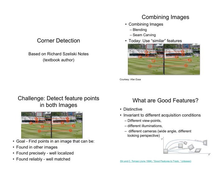
Combining Images

• Combining Images

– Blending – Seam Carving

• Today: Use “similar” features

Courtesy: Irfan Essa

Challenge: Detect feature points in both Images

• Goal - Find points in an image that can be:
• Found in other images
• Found precisely - well localized
• Found reliably - well matched

What are Good Features?

• Distinctive
• Invariant to different acquisition conditions

– Different view-points, – different illuminations, – different cameras (wide angle, different looking perspective)

X Y

t r a n s l a t i

• n

rotation affine scale perspective

Shi and C. Tomasi (June 1994). "Good Features to Track, ” (citeseer)

Find Corners

• Key property: In the region around a

corner, image gradient has

– two or more dominant directions

• Corners are repeatable and distinctive

Corner Detection: Basic Idea

flat region: no change in all directions edge: no change along the edge direction corner: significant change in all directions

• Recognize

the point by looking through a small window

• Shifting a

window in any direction should give a large change in intensity

Basic Idea

E(u,v) = w(x, y) I(x +u, y + v)− I(x, y) ⎡ ⎣ ⎤ ⎦

2 x,y

∑

Change of intensity for the shift [u,v]:

Intensity Shifted intensity Window function

• r

Window function w(x,y) = Gaussian 1 in window, 0 outside

• H. Moravec (1980). "Obstacle Avoidance and Navigation in the Real World by a Seeing Robot Rover"
• Computation of the change in appearance

by shifting the window by u,v:

I(x, y)

appearance by shifting the window

E(u, v)

Slide motivated by Alyosha Efros

E(0,0) E(3,2)

E(u,v) = w(x, y) I(x +u, y + v)− I(x, y) ⎡ ⎣ ⎤ ⎦

2 x,y

∑

M = X

x,y

w(x, y)  I2

x

IxIy IxIy I2

y

• M

E(u, v) ≈ ⇥ u v ⇤ M  u v

• Convert the above formula (uses Taylor

Series expansion) –

• M is matrix computed from image derivatives – M is also

called structure tensor

Familiar? These are just products of Component of the gradients Ix, Iy,

Intuition

• Treat gradient vectors as a set of (dx,dy)

points with a center of mass defined as being at (0,0).

• Fit an ellipse to that set of points via scatter

matrix

• Analyze ellipse parameters for varying case.

Courtesy: R. Collins, Penn State University Courtesy: R. Collins, Penn State University

λ1~λ2 = small λ1 large; λ2 = small λ1~λ2 = large

Harris Detector: Mathematics

[ ]

( , ) , u E u v u v M v ⎡ ⎤ ≅ ⎢ ⎥ ⎣ ⎦

Intensity change in shifting window: eigenvalue analysis λ1, λ2 – eigenvalues of M

direction of the slowest change direction of the fastest change

(λmax)-1/2 (λmin)-1/2

Ellipse E(u,v) = const

Harris Detector: Mathematics

λ1 λ2 Corner λ1 and λ2 are large,

λ1 ~ λ2;

E increases in all

directions

λ1 and λ2 are small; E is almost constant

in all directions

Edge λ1 >> λ2 Edge λ2 >> λ1 Flat region Classification of image points using eigenvalues of M:

Harris Detector: Mathematics

Measure of corner response:

( )

2

det trace R M k M = −

1 2 1 2

det trace M M λ λ λ λ = = +

(k – empirical constant, k = 0.04-0.06)

Harris Detector: Mathematics

λ1 λ2 Corner Edge Edge Flat

• R depends only on

eigenvalues of M

• R is large for a corner
• R is negative with large

magnitude for an edge

• |R| is small for a flat

region R > 0 R < 0 R < 0 |R| small

Harris Detector (Preview) `Detect Corners’

• The Algorithm:

– Compute Gaussian derivatives at each pixel – Compute matrix M in a ga – Find points with large corner response function R (R > threshold) – Take the points of local maxima of R (we are not matching corner to ‘another’ image’s corner Yet)

• C. Harris and M. Stephens (1988). "A combined corner and edge detector"

Proceedings of the 4th Alvey Vision Conference. pp 147--151

Harris Detector: Workflow Harris Detector: Workflow

Compute corner response R

Harris Detector: Workflow

Find points with large corner response: R>threshold

Harris Detector: Workflow

Take only the points of local maxima of R

Harris Detector: Workflow

Harris Detector: Summary

• Average intensity change in direction [u,v] can be

expressed as a bilinear form:

• Describe a point in terms of eigenvalues of M:

measure of corner response

• A good (corner) point should have a large intensity

change in all directions, i.e. R should be large positive

[ ]

( , ) , u E u v u v M v ⎡ ⎤ ≅ ⎢ ⎥ ⎣ ⎦

( )

2 1 2 1 2

R k λλ λ λ = − +

Harris Detector: Some Properties

• Rotation invariance

Ellipse rotates but its shape (i.e. eigenvalues) remains the same Corner response R is invariant to image rotation

Harris Detector: Some Properties

• Partial invariance to affine intensity

change

ü Only derivatives are used => invariance to intensity shift I → I + b ü Intensity scale: I → a I R x (image coordinate)

threshold

R x (image coordinate)

Harris Detector: Some Properties

• But: non-invariant to image scale!

All points will be classified as edges

Corner !

Harris Detector: Some Properties

• Quality of Harris detector for different

scale changes

Repeatability rate:

# correspondences # possible correspondences C.Schmid et.al. Evaluation of Interest Point Detectors. IJCV 2000

Models of Image Change

• Geometry

– Rotation – Similarity (rotation + uniform scale) – Affine (scale dependent on direction) valid for: orthographic camera, locally planar object

• Photometry

– Affine intensity change (I → a I + b)

Rotation Invariant Detection

• Harris Corner Detector

C.Schmid et.al. Evaluation of Interest Point Detectors. IJCV 2000

Reading

• https://en.wikipedia.org/wiki/Corner_detection

– See bibliography for additional resources

• Shi and C. Tomasi (1994). Good Features to Track

– http://citeseer.ist.psu.edu/viewdoc/summary?doi=10.1.1.135.7147

• Moravec (1980) Corner Detector (Ch 5-6) ( here ).
• Harris & Stephens (1998), A Corner & Edge Detector

– http://www.bmva.org/bmvc/1988/avc-88-023.pdf – Very readable.

• Mikolajczyk and Schmid (2001). “Indexing Based on Scale Invariant Interest Points”

– http://www.ee.surrey.ac.uk/CVSSP/Publications/papers/Mikolajczyk-ICCV-2001.pdf

• Lowe (2004) “Distinctive Image Features from Scale-Invariant Keypoints”. IJCV 2004

– http://people.eecs.berkeley.edu/~malik/cs294/lowe-ijcv04.pdf

• Search for “Features” on OpenCV site