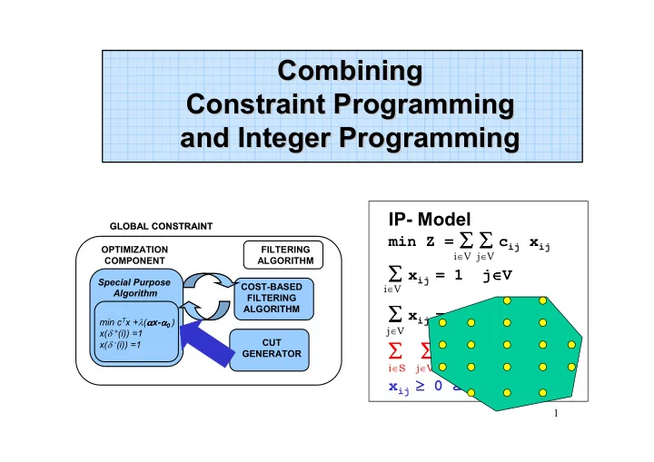
Combining Combining Constraint Programming Constraint Programming - - PowerPoint PPT Presentation

1

IP- Model

min Z = ∑

∑ ∑ ∑ ∑ ∑ ∑ ∑ cij xij ∑ ∑ ∑ ∑ xij = 1

j∈ ∈ ∈ ∈V

∑ ∑ ∑ ∑ xij = 1

i∈ ∈ ∈ ∈V

∑ ∑ ∑ ∑ ∑ ∑ ∑ ∑ xij ≥

≥ ≥ ≥ 1 S⊂ ⊂ ⊂ ⊂V S≠∅ ≠∅ ≠∅ ≠∅ xij ≥ ≥ ≥ ≥ 0 and integer

i∈V j∈V i∈V j∈V i∈S j∈V\S

Combining Combining Constraint Programming Constraint Programming and Integer Programming and Integer Programming

GLOBAL CONSTRAINT GLOBAL CONSTRAINT COST-BASED FILTERING ALGORITHM OPTIMIZATION COMPONENT FILTERING ALGORITHM min cTx +λ(α α α αx-α α α α0 ) x(δ +(i)) =1 x(δ -(i)) =1 Special Purpose Algorithm CUT GENERATOR

2

• CP on Finite Domains CP(FD): a programming paradigm

exploiting Constraint Satisfaction techniques

• A Constraint Satisfaction Problem (CSP) consists of:

– – a set of a set of variables variables ( (V V1

1,

, V V2

2,…,

,…,V Vn

n)

) – – a discrete domain a discrete domain ( (D D1

1,

,D D2

2,…,

,…,D Dn

n)

) for each variable for each variable – – a set of a set of constraints constraints on

• n te

te variables: variables: “relations among variables which represent a subset of the Cartesian product of the domains D1 x D2 x ... x Dn” Solution of a CSP Solution of a CSP: : an assignment of values to variables consistent with the constr an assignment of values to variables consistent with the constraints aints

E.

• E. Tsang

Tsang: “ : “Foundations Foundations of

• f Constraint

Constraint Satisfaction Satisfaction” ” Academic Academic Press,1992. Press,1992.

Constraint Programming (CP) Preliminaries

3

Each variable is involved in many constraints Any change in the domain of a single variable may propagate to other variables. Constraints agents view: during their lifetime, the constraints alternate their status between suspended and woken states (triggered by events). Example:

CP Preliminaries – interaction among constraints

X::[1..5], Y::[1..5], Z::[1..5] X = Y + 1 Y = Z + 1 X = Z - 1

4

X::[1..5], Y::[1..5], Z::[1..5] X = Y + 1 Y = Z + 1 X = Z - 1

– First propagation of X = Y + 1 yields

X::[2..5], Y::[1..4], Z::[1..5] X = Y + 1 is then suspended

5

– Second propagation of Y = Z + 1 yields X::[2..5], Y::[2..4], Z::[1..3] Y = Z + 1 is then suspended – The domain of Y has changed, X = Y + 1 is then awakened X::[3..5], Y::[2..4], Z::[1..3] X = Y + 1 is then suspended

6

– Third propagation of X = Z - 1 yields

FAILURE detected

X::[] Y::[2..4] Z::[1..3]

7

– Branching strategies define the way

• f partitioning the problem P into

easier subproblems P1, P2,…, Pn. – To each subproblem: apply again propagation. – New branches can be pruned because of the new information derived from the branching

CP Preliminaries – search

• Pruning all the infeasible values from variable domains often has the

same complexity as solving the original problem

• Propagation algorithms are then incomplete, i.e., when propagation is

stopped, still some values left in the variable domains can be inconsistent a SEARCH step is executed.

P Pn P4 … P3 P2 P1

8

variable selection value selection constraint propagation const. 1 const 2 const 3 continue

• n success

backtrack

• n failure

The search scheme

9

• What about the objective function?

As soon as a feasible solution of value Z* (say) is found, a new bounding constraint is added so as to impose that further solutions must have a better value: Z < Z* Hence, CP solves a sequence of feasibility problems, constrained to improve the objective function value. However: Z is in general the sum of the values assumed by several variables the propagation of the bounding constraint is typically very weak

CP Preliminaries: dealing with an objective function

10

Example: (ATSP) Asymmetric Traveling SalesmanProblem

Given

• a directed graph G=(V,A) with nodes 0,1,…, n-1
• arc costs cij

i j

cij

Find

• a Hamiltonian tour (= closed circuit passing exactly once

through all nodes) of minimum total cost

11

ATSP: a CP model

X0::D0, X1::D1,..., Xk::Dk path([X0,X1,…,Xk])

Given the directed graph G=(V,A), associate to each node i a variable Xi whose domain contains the next possible nodes in a simple path. saying that the assignment of variables X0,X1,…,Xk has to define a simple path involving all nodes 0,…,k. CP standard modules include the following path constraint:

12

The Asymmetric Travelling Salesman Problem (ATSP) can then be formulated through the CP path constraint as follows:

• one of the nodes, say node 0, is duplicated generating node n
• the constraint path([X0,X1,…,Xn]) is imposed

n i j

cij

13

ATSP: an IP model

A j i x S V S x V i x V j x To Subject x c Minimize

ij S i S j ij V j ij V i ij A j i ij ij

∈ ∀ >= ≠ ⊂ ∀ >= = ∈ ∀ = = ∈ ∀ =

∑∑ ∑ ∑ ∑

∈ ∉ ∈ ∈ ∈

) , ( integer subtours) (no : 1 1) (outdegree 1 1) (indegree 1 : :

) , (

solution the in j i iff xij ) , ( 1 =

i j

} 1 , { ∈

ij

x

14

Comparing the CP and IP models

Mapping

Xi = vj path ([X0, X1, ….., Xn]) Ci=cij xij=1 linear constr.s cij iff xij=1

CP- Model:

Xi::[v1,v2,…,vn] i=0..n-1 path([X0,X1,…,Xn]) Ci::[ci1,ci2,…,cin]i=0..n-1 Cn = 0; Xn = 0; C0+…+Cn-1 = Z minimize(Z)

IP- Model

min Z = ∑

∑ ∑ ∑ ∑ ∑ ∑ ∑ cij xij ∑ ∑ ∑ ∑ xij = 1

j∈ ∈ ∈ ∈V

∑ ∑ ∑ ∑ xij = 1

i∈ ∈ ∈ ∈V

∑ ∑ ∑ ∑ ∑ ∑ ∑ ∑ xij ≥

≥ ≥ ≥ 1 S⊂ ⊂ ⊂ ⊂V S≠∅ ≠∅ ≠∅ ≠∅ xij ≥ ≥ ≥ ≥ 0 and integer

i∈V j∈V i∈V j∈V i∈S j∈V\S

15

Pure IP vs Pure CP

Tight LP relaxation, easy feasibility: IP wins Almost useless LP relaxation, hard feasibility: CP wins

[ [red red,blue,green,yellow, ,blue,green,yellow,pink pink] ] [ [red red,blue,green,yellow, ,blue,green,yellow,pink pink] ]

V V1

1

V V2

2

V V3

3

V V5

5

V V4

4

≠ ≠ ≠ ≠ ≠ ≠ ≠ ≠ ≠ ≠ ≠ ≠ ≠ ≠ ≠ ≠ ≠ ≠

[ [red red,blue,green,yellow, ,blue,green,yellow,pink pink] ] [ [red red,blue,green,yellow, ,blue,green,yellow,pink pink] ]

16

CP+IP: preliminary results

• Although CP is not competitive for problems like TSP and

ATSP, the addition of an IP optimization component within the CP framework allows for the solution of instances of significantly larger size (Lodi et al., 2003)

TSP and ATSP instances pure AP AP + Lagrangean relaxation of cuts Instance Opt Time Fails Opt Time Fails Gr17 2085 0.39 511 2085 0.49 30 Fri26 937 0.82 725 937 0.71 80 Bays29 2020 4.12 4185 2020 1.20 403 Dantzig42 699 >300

• 699

5.55 1081 RY48P 14854* >300

• 14422

130.00 50K

• Pure CP gets stuck on problems with 15-20 nodes.