MA/CSSE 473 Day 22 Binary Heaps Heapsort Exam 2 Answers to - - PDF document

1

MA/CSSE 473 Day 22

Binary Heaps Heapsort Answers to student questions Exam 2 Tuesday, Nov 4 in class

Binary (max) Heap Quick Review

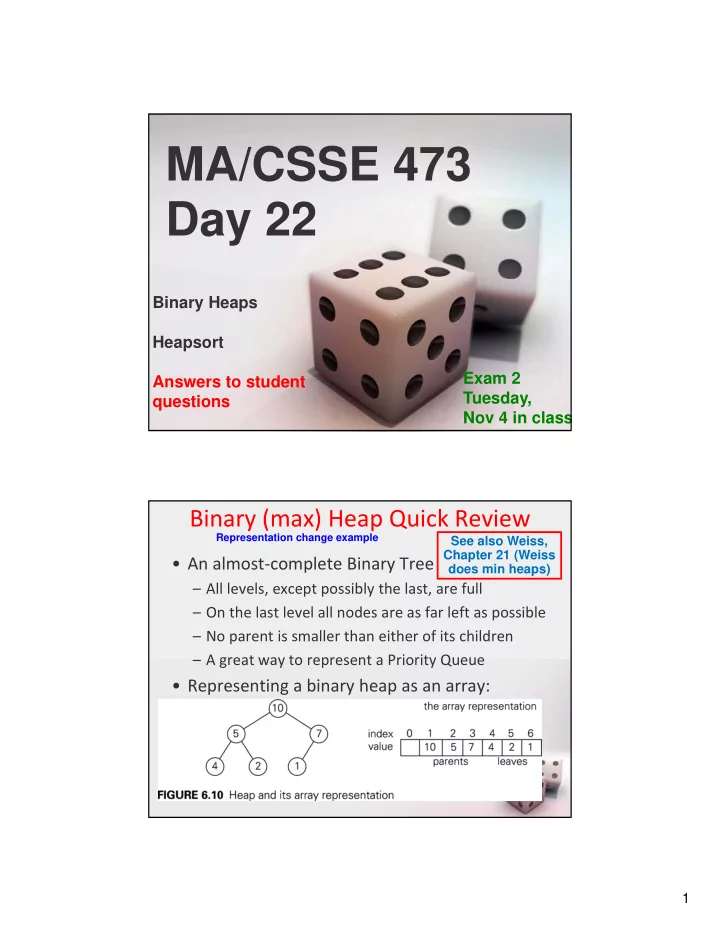
• An almost‐complete Binary Tree

– All levels, except possibly the last, are full – On the last level all nodes are as far left as possible – No parent is smaller than either of its children – A great way to represent a Priority Queue

• Representing a binary heap as an array:

See also Weiss, Chapter 21 (Weiss does min heaps)

Representation change example

2

Insertion and RemoveMax

• Insertion:

– Insert at the next position (end of the array) to maintain an almost‐complete tree, then "percolate up" within the tree to restore heap property.

• RemoveMax:

– Move last element of the heap to replace the root, then "percolate down" to restore heap property.

• Both operations are Ѳ(log n).
• Many more details (done for min‐heaps):

– http://www.rose‐ hulman.edu/class/csse/csse230/201230/Slides/18‐ Heaps.pdf

Heap utilitiy functions

Code is on-line, linked from the schedule page

3

HeapSort

• Arrange array into a heap. (details next slide)
• for i = n downto 2:

a[1]a[i], then "reheapify" a[1]..a[i‐1]

• Animation:

http://www.cs.auckland.ac.nz/software/AlgAni m/heapsort.html

• Faster heap building algorithm: buildheap

http://students.ceid.upatras.gr/~perisian/data _structure/HeapSort/heap_applet.html

HeapSort Code

4

Recap: HeapSort: Build Initial Heap

• Two approaches:

– for i = 2 to n percolateUp(i) – for j = n/2 downto 1 percolateDown(j)

• Which is faster, and why?
• What does this say about overall big‐theta

running time for HeapSort?

TRANSFORM AND CONQUER

Polynomial Evaluation Problem Reductiion

5

Recap: Horner's Rule

• We discussed it in class previously
• It involves a representation change.
• Instead of anxn + an‐1xn‐1 + …. + a1x + a0, which

requires a lot of multiplications, we write

• ( … (anx + an‐1)x + … +a1 )x + a0
• code on next slide

Recap: Horner's Rule Code

• This is clearly Ѳ(n).

6

Problem Reduction

• Express an instance of a problem in terms of an

instance of another problem that we already know how to solve.

• There needs to be a one‐to‐one mapping between

problems in the original domain and problems in the new domain.

• Example: In quickhull, we reduced the problem of

determining whether a point is to the left of a line to the problem of computing a simple 3x3 determinant.

• Example: Moldy chocolate problem in HW 9.

The big question: What problem to reduce it to? (You'll answer that one in the homework)

Least Common Multiple

• Let m and n be integers. Find their LCM.
• Factoring is hard.
• But we can reduce the LCM problem to the

GCD problem, and then use Euclid's algorithm.

• Note that lcm(m,n)∙gcd(m,n) = m∙n
• This makes it easy to find lcm(m,n)

7

Paths and Adjacency Matrices

• We can count paths from A to B in a graph by

looking at powers of the graph's adjacency matrix.

For this example, I used the applet from http://oneweb.utc.edu/~Christopher-Mawata/petersen2/lesson7.htm, which is no longer accessible

Linear programming

• We want to maximize/minimize a linear function

, subject to constraints, which are linear equations or inequalities involving the n variables x1,…,xn .

• The constraints define a region, so we seek to maximize

the function within that region.

• If the function has a maximum or minimum in the

region it happens at one of the vertices of the convex hull of the region.

• The simplex method is a well‐known algorithm for

solving linear programming problems. We will not deal with it in this course.

• The Operations Research courses cover linear

programming in some detail.



 n i i ix

c

1

8

Integer Programming

• A linear programming problem is called an

integer programming problem if the values of the variables must all be integers.

• The knapsack problem can be reduced to an

integer programming problem:

• maximize subject to the constraints

and xi {0, 1} for i=1, …, n

i n i iv

x



1







n i i i

W w x

1

SPACE‐TIME TRADEOFFS

Sometimes using a little more space saves a lot of time

9

Space vs time tradeoffs

• Often we can find a faster algorithm if we are

willing to use additional space.

• Examples: