} Input Correctness Output Rigorous, Unambiguous and - PDF document

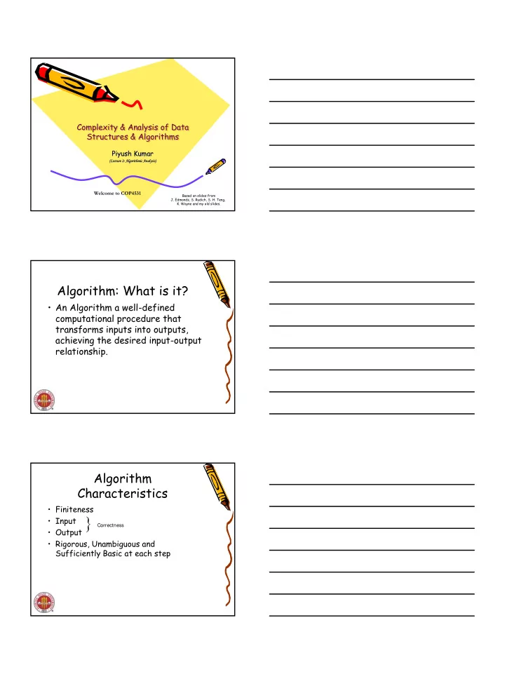
Complexity & Analysis of Data Complexity & Analysis of Data Complexity & Analysis of Data Structures & Algorithms Structures & Algorithms Structures & Algorithms Piyush Kumar Piyush Kumar (Lecture 2: Alg (Lecture 2: Alg (Lect (Lect e 2: Algorit e 2: Algorit rithmic An rithmic An mic Analys mic Analys alysis alysis is) is) Welcome to COP4531 Based on slides from J. Edmonds, S. Rudich, S. H. Teng, K. Wayne and my old slides. Algorithm: What is it? • An Algorithm a well-defined computational procedure that transforms inputs into outputs, achieving the desired input-output relationship. Algorithm Characteristics • Finiteness } • Input Correctness • Output • Rigorous, Unambiguous and Sufficiently Basic at each step 1

Applications? • WWW and the Internet • Computational Biology • Scientific Simulation • VLSI Design • Security • Automated Vision/Image Processing • Compression of Data • Databases • Mathematical Optimization Sorting • Input: • Input: Array A[1...n], of elements in arbitrary order • Output: Array A[1...n] of the same elements, but in increasing order • Given a teacher find all his/her students. • Given a student find all his/her teachers. The RAM Model • Analysis is performed with respect to a computational model • We will usually use a generic uniprocessor random-access machine (RAM) – All memory equally expensive to access – No concurrent operations – All reasonable instructions take unit time • Except, of course, function calls – Constant word size • Unless we are explicitly manipulating bits 2

Binary Search Initialize High < Low Failure Get Midpoint Adjust Low Adjust High > < Compare = Success Time and Space Complexity • Generally a function of the input size • E.g., sorting, multiplication – How we characterize input size depends: • Sorting: number of input items • Multiplication: total number of bits • Graph algorithms: number of nodes & edges • Etc Running Time • Number of primitive steps that are executed – Except for time of executing a function call most statements roughly require the same amount of time • y = m * x + b • c = 5 / 9 * (t - 32 ) • z = f(x) + g(y) • We can be more exact if need be 3

Analysis • Worst case – Provides an upper bound on running time – An absolute guarantee • Average case – Provides the expected running time – Very useful, but treat with care: what is “average”? • Random (equally likely) inputs • Real-life inputs Binary Search Analysis • Order Notation • Upper Bounds • Search Time = ?? • A better way to look at it, Binary Search Trees In this course • We care most about asymptotic performance – How does the algorithm behave as the problem size gets very large? • Running time • Memory/storage requirements • Bandwidth/power requirements/logic gates/etc. 4

2.1 Computational Tractability "For me, great algorithms are the poetry of computation. Just like verse, they can be terse, allusive, dense, and even mysterious. But once unlocked, they cast a brilliant new light on some aspect of computing." - Francis Sullivan Computational Tractability As soon as an Analytic Engine exists, it will necessarily guide the future course of the science. Whenever any result is sought by its aid, the question will arise - By what course of calculation can these results be arrived at by the machine in the shortest time? - Charles Babbage Charles Babbage (1864) Analytic Engine (schematic) Polynomial-Time • Brute force. For many non-trivial problems, there is a natural brute force search algorithm that checks every possible solution. Typically takes 2 N time or worse for inputs of size N. – – Unacceptable in practice. n ! for stable matching with n men and n women • Desirable scaling property. When the input size doubles, the algorithm should only slow down by some constant factor C. There exists constants c > 0 and d > 0 such that on every input of size N, its running time is bounded by c N d steps. • Def. An algorithm is poly-time if the above scaling property holds. choose C = 2 d 5

Worst-Case Analysis • Worst case running time. Obtain bound on largest possible running time of algorithm on input of a given size N. – Generally captures efficiency in practice. – Draconian view, but hard to find effective alternative. • Average case running time. Obtain bound on running time of algorithm on random input as a function of input size N. – Hard (or impossible) to accurately model real instances by random distributions. – Algorithm tuned for a certain distribution may perform poorly on other inputs. Worst-Case Polynomial-Time • Def. An algorithm is efficient if its running time is polynomial. • Justification: It really works in practice! Although 6.02 × 10 23 × N 20 is technically poly-time, it would be useless – in practice. – In practice, the poly-time algorithms that people develop almost always have low constants and low exponents. – Breaking through the exponential barrier of brute force typically exposes some crucial structure of the problem. • Exceptions. – Some poly-time algorithms do have high constants and/or exponents, and are useless in practice. – Some exponential-time (or worse) algorithms are widely used because the worst-case instances seem to be rare. simplex method Unix grep Why It Matters 6

2.2 Asymptotic Order 2.2 Asymptotic Order 2.2 Asymptotic Order of Growth of Growth of Growth Why not do Exact Analysis? • It is difficult to be exact. • Results are most of the time too complicated and irrelevant. Order Notation 7

Asymptotic Order of Growth • Upper bounds. T(n) is O(f(n)) if there exist constants c > 0 and n 0 ≥ 0 such that for all n ≥ n 0 we have T(n) ≤ c · f(n). • Lower bounds. T(n) is Ω (f(n)) if there exist constants c > 0 and n 0 ≥ 0 such that for all n ≥ n 0 we have T(n) ≥ c · f(n). • Tight bounds. T(n) is Θ (f(n)) if T(n) is both O(f(n)) and Ω (f(n)). Ex: T(n) = 32n 2 + 17n + 32. • – T(n) is O(n 2 ), O(n 3 ), Ω (n 2 ), Ω (n), and Θ (n 2 ) . – T(n) is not O(n), Ω (n 3 ), Θ (n), or Θ (n 3 ). Notation • Slight abuse of notation. T(n) = O(f(n)). – Asymmetric: • f(n) = 5n 3 ; g(n) = 3n 2 • f(n) = O(n 3 ) = g(n) • but f(n) ≠ g(n). – Better notation: T(n) ∈ O(f(n)). • Meaningless statement. Any comparison-based sorting algorithm requires at least O(n log n) comparisons. – Statement doesn't "type-check." – Use Ω for lower bounds. Properties • Transitivity. – If f = O(g) and g = O(h) then f = O(h). – If f = Ω (g) and g = Ω (h) then f = Ω (h). – If f = Θ (g) and g = Θ (h) then f = Θ (h). • Additivity. – If f = O(h) and g = O(h) then f + g = O(h). – If f = Ω (h) and g = Ω (h) then f + g = Ω (h). – If f = Θ (h) and g = O(h) then f + g = Θ (h). 8

Asymptotic Bounds for Some Common Functions Polynomials. a 0 + a 1 n + … + a d n d is Θ (n d ) if a d > 0. • • Polynomial time. Running time is O(n d ) for some constant d independent of the input size n. • Logarithms. O(log a n) = O(log b n) for any constants a, b > 0. can avoid specifying the base • Logarithms. For every x > 0, log n = O(n x ). log grows slower than every polynomial Exponentials. For every r > 1 and every d > 0, n d = O(r n ). • every exponential grows faster than every polynomial The world of O… • F(n) = O(F(n)) • c O(f(n)) = O(f(n)) • O(F(n)) = O(O(F(n))) • O(f(n)+g(n)) = O( max(f(n),g(n)) ) • O(f(n)) O(g(n)) = O( f(n) g(n) ) • O( f(n) g(n) ) = f(n) O( g(n) ) 2.4 A Survey of Common 2.4 2.4 A Survey of Common A Survey of Common Running Times Running Times Running Times 9

Linear Time: O(n) • Linear time. Running time is at most a constant factor times the size of the input. max ← a 1 for i = 2 to n { if (a i > max) max ← a i } • Computing the maximum. Compute maximum of n numbers a 1 , …, a n . Linear Time: O(n) • Merge. Combine two sorted lists A = a 1 ,a 2 ,…,a n with B = b 1 ,b 2 ,…,b n into sorted whole. i = 1, j = 1 while (both lists are nonempty) { if (a i ≤ b j ) append a i to output list and increment i else(a i ≤ b j )append b j to output list and increment j } append remainder of nonempty list to output list • Claim. Merging two lists of size n takes O(n) time. • Pf. After each comparison, the length of output list increases by 1. O(n log n) Time • O(n log n) time. Arises in divide-and-conquer algorithms. also referred to as linearithmic time • Sorting. Mergesort and heapsort are sorting algorithms that perform O(n log n) comparisons. • Largest empty interval. Given n time-stamps x 1 , …, x n on which copies of a file arrive at a server, what is largest interval of time when no copies of the file arrive? • O(n log n) solution. Sort the time-stamps. Scan the sorted list in order, identifying the maximum gap between successive time-stamps. 10