Implications of Big Data for Statistics Instruction 17 Nov 2013 - PDF document

Implications of Big Data for Statistics Instruction 17 Nov 2013 Teaching Introductory Business Statistics Implications of Big Data to Undergraduates in an Era of Big Data for Statistics Instruction “The integration of business, Big Data and Mark L. 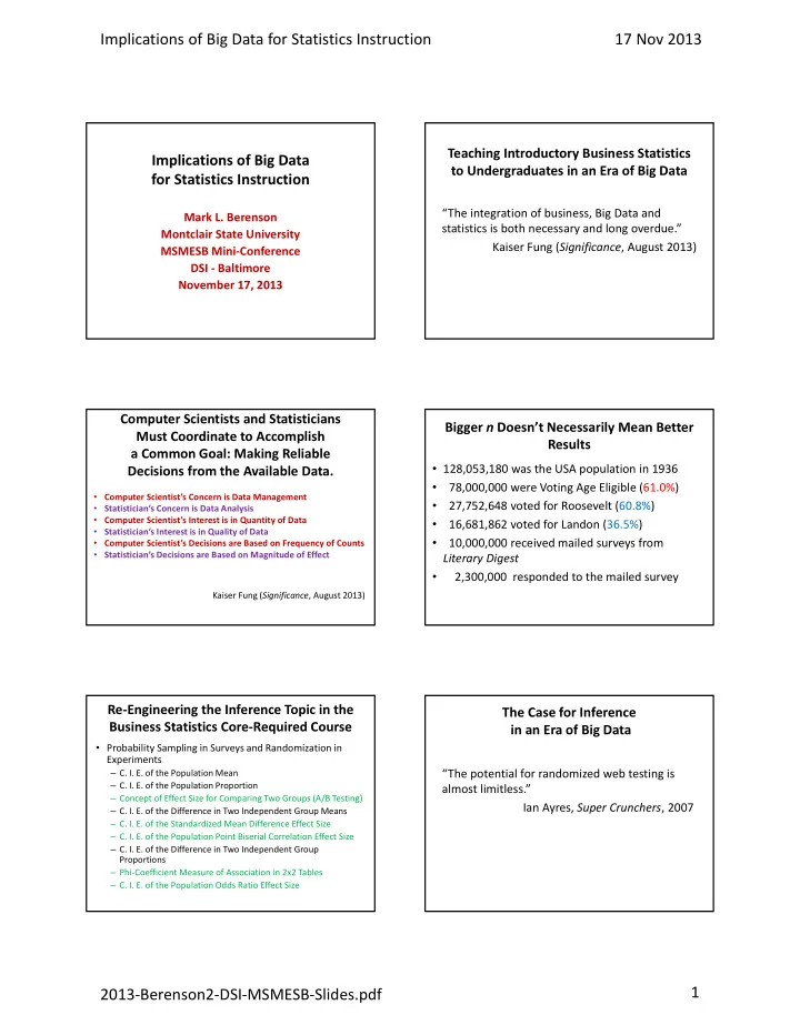Berenson statistics is both necessary and long overdue.” Montclair State University Kaiser Fung ( Significance , August 2013) MSMESB Mini ‐ Conference DSI ‐ Baltimore November 17, 2013 Computer Scientists and Statisticians Bigger n Doesn’t Necessarily Mean Better Must Coordinate to Accomplish Results a Common Goal: Making Reliable • 128,053,180 was the USA population in 1936 Decisions from the Available Data. • 78,000,000 were Voting Age Eligible (61.0%) • Computer Scientist’s Concern is Data Management • 27,752,648 voted for Roosevelt (60.8%) • Statistician’s Concern is Data Analysis • Computer Scientist’s Interest is in Quantity of Data • 16,681,862 voted for Landon (36.5%) • Statistician’s Interest is in Quality of Data • • Computer Scientist’s Decisions are Based on Frequency of Counts 10,000,000 received mailed surveys from • Statistician’s Decisions are Based on Magnitude of Effect Literary Digest • 2,300,000 responded to the mailed survey Kaiser Fung ( Significance , August 2013) Re ‐ Engineering the Inference Topic in the The Case for Inference Business Statistics Core ‐ Required Course in an Era of Big Data • Probability Sampling in Surveys and Randomization in Experiments – C. I. E. of the Population Mean “The potential for randomized web testing is – C. I. E. of the Population Proportion almost limitless.” – Concept of Effect Size for Comparing Two Groups (A/B Testing) Ian Ayres, Super Crunchers , 2007 – C. I. E. of the Difference in Two Independent Group Means – C. I. E. of the Standardized Mean Difference Effect Size – C. I. E. of the Population Point Biserial Correlation Effect Size – C. I. E. of the Difference in Two Independent Group Proportions – Phi ‐ Coefficient Measure of Association in 2x2 Tables – C. I. E. of the Population Odds Ratio Effect Size 1 2013 ‐ Berenson2 ‐ DSI ‐ MSMESB ‐ Slides.pdf

Implications of Big Data for Statistics Instruction 17 Nov 2013 The Case for Inference The Case for Inference in an Era of Big Data in an Era of Big Data “Any large organization that is not exploiting both “Testing is a road that never ends. Tastes regression and randomization is presumptively change. What worked yesterday will not work missing value. Especially in mature industries, tomorrow. A system of periodic retesting with where profit margins narrow, firms ‘ competing on randomized trials is a way to ensure that your analytics’ will increasingly be driven to use both marketing efforts remain optimized.” tools to stay ahead. … Randomization and Ian Ayres, Super Crunchers , 2007 regression are the twin pillars of Super Crunching.” Ian Ayres, Super Crunchers , 2007 The Problem with Hypothesis Testing The Case for Effect Size Measures to in an Era of Big Data Replace Hypothesis Testing (NHST) in an Era of Big Data • H. Jeffreys (1939) and D.V. Lindley (1957) point out that any observed trivial difference will The use of NHST “has caused scientific research become statistically significant if the sample workers to pay undue attention to the results of sizes are large enough. the tests of significance that they perform on their data and too little attention on the magnitude of the effects they are investigating.“ Frank Yates ( JASA , 1951) The Case for Effect Size Measures to The Case for Effect Size Measures to Replace Hypothesis Testing (NHST) Replace Hypothesis Testing (NHST) in an Era of Big Data in an Era of Big Data “In many experiments, it seems obvious that the “Estimates of appropriate effect sizes and [their] different treatments must produce some difference, confidence intervals are the minimum expectations however small, in effect. Thus the hypothesis that for all APA journals.” there is no difference is unrealistic. The real Publication Manual of the APA (2010) problem is to obtain estimates of the size of the differences.” George W. Cochran and Gertrude M. Cox, Experimental Design , 2 nd Ed., (1957) 2 2013 ‐ Berenson2 ‐ DSI ‐ MSMESB ‐ Slides.pdf

Implications of Big Data for Statistics Instruction 17 Nov 2013 What an Effect Size Measures Why Effect Size is Important • When comparing differences in the means of Knowing the magnitude of an effect enables an two groups the effect size quantifies the assessment of the practical importance of the magnitude of that difference. results. • When studying the association between two variables the effect size measures the strength of the relationship between them. Early Researchers Why the C.I.E. is Superior to the NHST in the Study of Effect Size • Jacob Cohen (NYU) • A confidence interval estimate is superior to a • Gene Glass (Johns Hopkins) hypothesis test because it gives the same • Larry Hedges (University of Chicago) information and provides a measure of precision. • Ingram Olkin (Stanford) • Robert Rosenthal (Harvard) • Donald Rubin (Harvard) ‐‐‐‐‐‐‐‐‐‐‐‐‐‐‐‐‐‐‐‐‐‐‐‐‐‐‐‐‐‐‐‐‐‐‐‐‐‐‐‐‐‐‐‐‐‐‐‐‐‐‐ • Ken Kelley (Notre Dame) Necessity for Standardization A C.I.E. is an Effect Size Measure • If common scales are being used to measure • If unfamiliar scales are being used to measure the outcome variables a regular confidence the outcome variables, in order to make interval estimate (of the unstandardized mean comparisons with results from other, similar difference) provides a representation of the studies done using different scales, a effect size. transformation to standardized units will be more informative and a confidence interval estimate of the standardized mean difference provides a representation of the effect size. 3 2013 ‐ Berenson2 ‐ DSI ‐ MSMESB ‐ Slides.pdf

Implications of Big Data for Statistics Instruction 17 Nov 2013 What Standardization Achieves Cohen’s Effect Size Classifications • Cohen (1992) developed effect size cut points of • A standardized effect size removes the sample .2, .5 and .8, respectively, for small , medium and size of the outcome variable from the effect large effects for standardized mean differences. estimate, producing a dimensionless • Cohen classified effect size cut points of .1, .3 standardized effect that can be compared and .5, respectively, for small , medium and large across different but related outcome variables effects for correlations. in other studies. • Cohen described a medium effect size as one in which the researcher can visually see the gains from treatment E above and beyond that of treatment C. Bonett’s Effect Size C. I. E. C. I. E. for the Difference in Means * Assuming Unequal Variances of Two Independent Groups *Assuming Unequal Variances *Assuming Equal Sample Sizes Bonett’s (2008) approximate (1 -  ) 100% confidence interval estimate of the population *Assuming Equal Sample Sizes standardized mean difference effect size  is given by   ˆ ˆ 1 / 2   (  ) As the sample sizes increase approaches so that for very large n and n an Z Var t Z  / 2   / 2 / 2 E C where the estimate of  is approximate (1 -  ) 100% confidence interval estimate of the difference in the population    E  Y Y means ( ) is given by ˆ   E C  ˆ C 1 / 2  2  2  ( ) 1 / 2 S S . The variance of the statistic  ˆ proposed by Bonett       and ˆ  E C  when 2 2 n n S S 2 E C     ( )  E C  Y Y Z  / 2 E C  n  reduces to * ˆ  2 ( 4  4 ) S S 2 ˆ (  )   Var E C where the equal sample sizes n and n are given by n .  8  ˆ 4 (  1 ) ( 1 ) n n * * * E C when the equal sample sizes n and n are represented by n . * E C Rosenthal’s Effect Size Confidence Interval Rosenthal’s Effect Size Confidence Interval for the Point Biserial Correlation Coefficient for the Point Biserial Correlation Coefficient An approximate (1 -  ) 100% confidence interval estimate of the population point biserial  coefficient of correlation is obtained using the Fisher Z transformation where When the sample sizes are equal the point biserial correlation coefficient r is obtained from pb r pb  1   r  pb Z 0 . 5 ln     Y Y r  1   r   E C pb r pb 2 S Y and the standard error is 1 / 2 1 / 2  2   1  n  i  2   ( )  S   Y Y Z   3  ij r  n n  Y Y   E C    1  1 where E C and i j . Y S 2 Y    n n The confidence interval limits for this are obtained from  so that Z Z S  E C  r  / 2 Z r        1 / 2 1 r 1  0 . 5 ln  pb    Z   / 2   ˆ are related as follows:  1  3 Also, for very large sample size, r and   r   n n  pb E C pb and the approximate (1 -  ) 100% confidence interval estimate of the population  is obtained  ˆ 2 pb r ˆ by taking the antilogs of the above lower and upper limits. The conversions for each limit are  and   pb r     pb ˆ 1 / 2  1 / 2  2  4 1 2 given by r pb 2 Z  1 e r    pb 2 Z 1 e r 4 2013 ‐ Berenson2 ‐ DSI ‐ MSMESB ‐ Slides.pdf