Topics of the day Logistic regression and generalized linear models - - PowerPoint PPT Presentation

Logistic regression and generalized linear models

Rasmus Waagepetersen Department of Mathematics Aalborg University Denmark November 5, 2019

1 / 27

Topics of the day

◮ Logistic regression ◮ Overdispersion ◮ Logistic regression with random effects

2 / 27

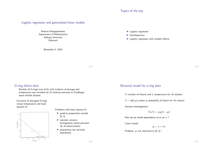
O-ring failure data

Number of O-rings (out of 6) with evidence of damage and temperature was recorded for 23 missions previous to Challenger space shuttle disaster. Fractions of damaged O-rings versus temperature and least squares fit:

40 50 60 70 80 0.0 0.2 0.4 0.6 0.8 temperature Fraction damaged

Problems with least squares fit: ◮ predicts proportions outside [0, 1]. ◮ assumes variance homogeneity (same precision for all observations). ◮ proportions not normally distributed.

3 / 27

Binomial model for o-ring data

Yi number of failures and ti temperature for ith mission. Yi ∼ b(6, pi) where pi probability of failure for ith mission. Variance heterogeneity: VarYi = nipi(1 − pi) How do we model dependence of pi on ti ? Linear model: pi = α + βti Problem: pi not restricted to [0, 1] !

4 / 27

Logistic regression

Consider logit transformation: η = logit(p) = log( p 1 − p) Note: logit injective function from ]0, 1[ to R. Hence we may apply linear model to η and transform back: η = α + βt ⇔ p = exp(α + βt) exp(α + βt) + 1 Note: p guaranteed to be in ]0, 1[

5 / 27

Plots of logit, inverse logit, and probit

0.0 0.2 0.4 0.6 0.8 1.0 −6 −4 −2 2 4 6 p logit(p) −10 −5 5 10 0.0 0.2 0.4 0.6 0.8 1.0 eta invlogit(eta)

−10 −5 5 10 0.0 0.2 0.4 0.6 0.8 1.0 eta p logistisk probit

Probit transformation: pi = Φ(ηi) where Φ cumulative distribution function of standard normal variable (Φ(u) = P(U ≤ u).) Regression parameter for logistic roughly 1.8 times regression parameter for probit since Φ more steep than inverse logit.

6 / 27

Logistic regression and odds

Odds for a failure in ith mission is

• i =

pi 1 − pi = exp(ηi) and odds ratio is

• i
• j

= exp(ηi − ηj) = exp(β(ti − tj)) Example: to double odds we need 2 = exp(β(ti − tj)) ⇔ ti − tj = log(2)/β

7 / 27

Estimation

Likelihood function for simple logistic regression logit(pi) = α + βxi: L(α, β) =

• i

pyi

i (1 − pi)ni−yi

where pi = exp(α + βxi) 1 + exp(α + βxi) MLE (ˆ α, ˆ β) found by iterative maximization (Newton-Raphson) More generally we may have multiple explanatory variables: logit(pi) = β1x1i + . . . + βpxpi

8 / 27

Deviance

Predicted observation for current model: ˆ yi = ni ˆ pi logitˆ pi = ˆ β1x1i + . . . + ˆ βpxpi Saturated model: no restrictions on pi so ˆ psat

i

= yi/ni and ˆ ysat

i

= yi (perfect fit). Residual deviance D is -2 times the log of the ratio between L(ˆ β1, . . . , ˆ βp) and likelihood Lsat for the saturated model. D = 2

n

• i=1

[yi log(yi/ˆ yi) + (ni − yi) log((ni − yi)/(ni − ˆ yi))] If ni not too small D ≈ χ2(n − p) where p is the number of parameters for current model. If this is the case, D may be used for goodness-of-fit assessment. Null deviance is log ratio between maximum likelihood for model with only intercept and Lsat.

9 / 27

Pearson’s X 2: X 2 =

n

• i=1

(yi − ni ˆ pi)2 ni ˆ pi(1 − ˆ pi) is asymptotically equivalent alternative to D.

10 / 27

Logistic regression in R

> out=glm(cbind(damage,6-damage)~temp,family=binomial(logit)) > summary(out) ... Coefficients: Estimate Std. Error z value Pr(>|z|) (Intercept) 11.66299 3.29626 3.538 0.000403 *** temp

• 0.21623

0.05318

• 4.066 4.78e-05 ***

... Null deviance: 38.898

• n 22

degrees of freedom Residual deviance: 16.912

• n 21

degrees of freedom ... ni = 6 so residual deviance approximately χ2(21) Residual deviance not large compared with numbers of degrees of freedom.

11 / 27

Generalized linear models

Suppose Z is random variable with expectation EZ = µ ∈ M where M ⊂ R. Idea: use invertible link function g : M → R and apply linear modelling to η = g(µ). Binomial data: Z = Y /n, Y ∼ b(n, p). µ = p ∈ M =]0, 1[. g(·) e.g. logistic or probit. Poisson data: Z ∼ pois(λ). µ = λ > 0. g e.g. log. Many other possibilities (McCullagh and Nelder, Faraway, Dobson) e.g. gamma distribution and inverse Gaussian for positive continuous data. For binomial and Poisson, VarZ = V (µ) determined by µ: V (µ) = µ(1 − µ)/n and V (µ) = µ, respectively.

12 / 27

Overdispersion

In some applications we see larger variability in the data than predicted by variance formulas for binomial. This is also sometimes revealed by large residual deviance or X 2 relative to degrees of freedom. Reason may either systematic defiency of model (misspecified mean structure) or overdispersion, i.e. variance of observations larger than model predicts. Overdispersion may be caused e.g. by genetic variation between subjects, variation between batches in laboratory experiments, or variation in environment in agricultural trials. There are various ways to handle overdispersion - we will focus on a model based approach: generalized linear mixed models.

13 / 27

Wheezing data

The wheezing (Ohio) data has variables resp (binary indicator of wheezing status), id, age (of child), smoke (binary, mother smoker

• r not).

Aggregated data: (black=smoke, red=no smoke)

• −2.0

−1.5 −1.0 −0.5 0.0 0.5 1.0 0.00 0.05 0.10 0.15 0.20 age Wheeze proportin

• 14 / 27

Let Yij denote wheezing status of ith child at jth age. Assuming Yij is b(pij, 1) we try logistic regression logit(pij) = β0 + β1agej + β2smokei Assuming independence between observations from the same child, and letting Yi· be the sum of observations from ith child, VarYi· =Var(Yi1 + Yi2 + Yi3 + Yi4) = VarYi1 + VarYi2 + VarYi3 + VarYi4 =pi1(1 − pi1) + pi2(1 − pi2) + pi3(1 − pi3) + pi4(1 − pi4) Note: same variance of Yi· for all children with same value of smoke. We can calculate above theoretical variance from fitted model and compare with empirical variances. Smoke=0: theoretical: 0.58 empirical: 1.22. Smoke=1: theoretical: 0.48 empirical: 0.975

15 / 27

Issue: observations from same child are correlated - if we know first observation is non-wheeze then very likely three remaining

• bservations non-wheeze too.

Correlation can be due to genetics or the environment (more or less polluted) for the child. Explicit model these effects using random effect: logit(pij) = β0 + β1agej + β2smokei + Ui where Ui are N(0, τ 2) and independent among children. Such a model can be fitted by the R-procedure glmer with syntax very close related to lmer and glm

16 / 27

Logistic regression

> fit=glm(resp~age+smoke,family=binomial,data=ohio) Coefficients: Estimate Std. Error z value Pr(>|z|) (Intercept) -1.88373 0.08384 -22.467 <2e-16 *** age

• 0.11341

0.05408

• 2.097

0.0360 * smoke 0.27214 0.12347 2.204 0.0275 *

• Signif. codes:

0 ’***’ 0.001 ’**’ 0.01 ’*’ 0.05 ’.’ 0.1 ’ ’ 1 Null deviance: 1829.1

• n 2147

degrees of freedom Residual deviance: 1819.9

• n 2145

degrees of freedom According to above results, age and smoke both significant at the 5% level.

17 / 27

χ2 distribution of deviance residual not trustworthy here since ni = 1. We can increase ni by aggregrating over 8 categories for age × smoke but then variability between children hidden.

18 / 27

Mixed model analysis

> fiter=glmer(resp~age+smoke+(1|id),family=binomial,data=ohio) > summary(fiter) Random effects: Groups Name Variance Std.Dev. id (Intercept) 5.491 2.343 Number of obs: 2148, groups: id, 537 Fixed effects: Estimate Std. Error z value Pr(>|z|) (Intercept) -3.37396 0.27496 -12.271 <2e-16 *** age

• 0.17677

0.06797

• 2.601

0.0093 ** smoke 0.41478 0.28705 1.445 0.1485 Now only age is significant on the 5% level. Note large variance 5.491 for the Ui.

19 / 27

Interpretation of variance of random effects

Variance 5.491 corresponds to standard deviation 2.343. This means 95% probability interval for Ui is [−4.686, 4.686]. Large part of the variation explained by the Ui relative to the fixed effects.

20 / 27

Interpretation in terms of marginal variance ?

For logistic regression with random effects, the variance of an

• bservation Yij is

VarYij = Epi(1 − pi) + Varpi (1) where the expectation and variance is with respect to Ui in pi = exp(α + βzi + Ui) 1 + exp(α + βzi + Ui) There is no simple formula for this variance. Here pi(1 − pi) is the conditional variance of Yij given Ui - but this can not be evaluated since Ui is unobserved.

21 / 27

Interpretation in terms of odds

The odds are Oi = pi 1 − pi = exp(α + βzi + Ui) and the odds ratio between individuals i and j is Oi Oj = exp(β(zi − zj) + Ui − Uj) where Ui − Uj ∼ N(0, 2τ 2). Larsen et al. (2000) suggested to consider the median summary MOR = exp[β(zi−zj)+MED(|Ui−Uj|)] = exp[β(zi−zj)] exp[ √ 2τ0.6744)] between individuals i and j. Here factor exp[ √ 2τ0.6744)] is median odds ratio between the individual with highest random effect and the individual with lowest random effect (note we consider absolute value |Ui − Uj|).

22 / 27

95% intervals for probabilities or odds

Ui is between −1.96τ and 1.96τ with 95% probability. Hence odds Oi in interval [exp(α + βzi − 1.96τ); exp(α + βzi + 1.96τ)] with probability 95%. For probability pi the interval is

• exp(α + βzi − 1.96τ)

1 + exp(α + βzi − 1.96τ); exp(α + βzi + 1.96τ) 1 + exp(α + βzi + 1.96τ)

• 23 / 27

Wheezing data

E.g. with τ = 2.343 we get MOR=9.34. That is, keeping all fixed factors equal, for two randomly picked children, the median odds ratio between the child with highest random effect and the child with lowest random effect is 9.34. For child of centered age 0 and with smoking mother the 95% interval for wheezing is

• exp(−3.37 + 0.41 − 1.96 ∗ 2.34)

1 + exp(−3.37 + 0.41 − 1.96 ∗ 2.34); exp(−3.37 + 0.41 + 1.96 ∗ 2.34) 1 + exp(−3.37 + 0.41 + 1.96 ∗ 2.34)

• = [0.00; 0.84]

Mean probability (by Monte Carlo) is 0.16. Emphasizes the large individual specific effects.

24 / 27

Summary

◮ logistic regression very useful for binary data ◮ in some applications there is evidence of overdispersion (extra variance) ◮ easy to add random effects to model sources of overdispersion and thereby correctly model correlation between observations e.g. for same subject. ◮ thereby we get more trustworthy standard deviations for fixed effects estimates. ◮ disadvantage: not easy to interpret random effects variances in terms of variances and correlations of the response variable Yi. ◮ likelihood function very complicated Next time: computation of the likelihood (how does glmer work ?)

25 / 27

Exercises

• 1. Show that the probit model for binary data may be viewed as

a latent variable model where Y = 1[U < a + bx] for a latent standard normal variable U. The latent variable could e.g. correspond to susceptibility to an insecticide if Y represents dead/alive for an insect subjected to an insecticide dose x.

• 2. The wheezing data may be aggregated according to the

groups given by age and smoke (the aggregated data set is available at the web-page). Compare logistic regression analyses for the original and aggregated data.

• 3. The variance of a (standard) logistic distribution is π2/3.

Argue why this implies that a logistic regression with parameter β roughly corresponds to a probit regression with parameter β

√ 3 π ≈ β/1.8

26 / 27

• 4. An experiment was designed to assess the effect of different

stocks on the robustness of cherry flowers to frost. For 20 cherry trees of 5 different stock varieties, three branches were sampled and on each branch the status of 5 buds (dead=1 or alive=0) were recorded. The data are available as cherries_red.txt.

4.1 Fit a logistic model with systematic STOCK and BRANCHNR effects and with random BRANCHID and TREEID effects. Is there scope for simplification of the random part of the model ? 4.2 What can you conclude about the STOCK effects ? 4.3 Is there a BRANCHNR effect ? Does this make sense ?

• 5. Verify the variance expression (1).
• 6. Suppose that X1 and X2 are independent N(0, τ 2). Show that

the median of |X1 − X2| is √ 2τ0.6744. Hint: consider first median of (X1 − X2)2 which has a well-known distribution.

27 / 27