Implementation Issues More from Interface point of view V Eye Y - - PowerPoint PPT Presentation

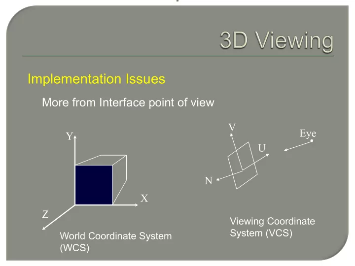
Implementation Issues

More from Interface point of view

Y Z X Eye N V U

World Coordinate System (WCS) Viewing Coordinate System (VCS)

View Coordinate System (VCS)

Viewing coordinate system

• Position and orientation of the view plane
• Extent of the view plane (window)
• Position of the eye

View Plane

• View Reference Point (VRP): the origin of VCS

specified as (rx , ry, rz) in WCS: center of the scene

• Normal to the view plane (nx , ny, nz )

View Plane

• Normal Direction (View Plane Normal

VPN) n (nx ,ny ,nz) User may provide normalized vector e.g. nx = sin φ cos θ ny = sin φ sin θ nz = cos φ

Z Y θ r X φ

View Coordinate System (VCS)

View Plane

• Direction v

v is a unit vector intuitively corresponding to “up” vector “up” vector is specified by the user in WCS

n up up’ v

up’ = up – (up.n)n v = up’ / |up’|

• Direction u

u = n x v ( Left Handed)

View Coordinate System (VCS)

Window and Eye

• Window : left, right, bottom,top (wl,wr,wb,wt)

generally is centered at VRP (origin)

• Eye : e = (eu,ev,en)

Typically e = (0,0,-E)

View Coordinate System (VCS)

u e wt wb wr wl n v

Transformation from WCS to VCS

r b a r v u b a y x + = + ⎟ ⎠ ⎞ ⎜ ⎝ ⎛ = M ) ( ) ( ) (

(x, y) X Y O O’ u v r

Transformation from WCS to VCS

Point object is represented as

• (a,b,c) in VCS
• (x,y,z) in WCS

⎥ ⎥ ⎥ ⎦ ⎤ ⎢ ⎢ ⎢ ⎣ ⎡ = ⎥ ⎥ ⎥ ⎦ ⎤ ⎢ ⎢ ⎢ ⎣ ⎡ =

z y x z y x z y x

n n n v v v u u u n v u M

[ ] [ ] [ ]

T

M r p M r p c b a r M c b a z y x p ) ( ) (

1

− = − = + = =

−

Transformation from WCS to VCS

Conversion from one coordinate system to another Therefore a=(p-r).u, b=(p-r).v, c=(p-r).n

[ ] [ ] [ ]

T

M r p M r p c b a r M c b a z y x p ) ( ) (

1

− = − = + = =

−

Conversion from one coordinate system to another ⎥ ⎥ ⎥ ⎦ ⎤ ⎢ ⎢ ⎢ ⎣ ⎡ = ⎥ ⎥ ⎥ ⎦ ⎤ ⎢ ⎢ ⎢ ⎣ ⎡ =

z y x z y x z y x

n n n v v v u u u n v u M

• (a,b,c) in VCS
• (x,y,z) in WCS

Where

3D Viewing Interface (Revisit)

Set up

Set up

Steps

• 1. Define the view reference point (VRP) = r
• 2. Obtain M defining u, v, n
• 3. Define the position of eye (in VCS)

e = ( eu, ev, en) typically ( 0, 0, -E ) corresponding point in WCS will be eye = ( 0, 0, -E ) M + r

• 4. Define the window and the pixel location.

Set up

rows : 0 to MAXROW cols : 0 to MAXCOL (i,j)th pixel : (ui, vj, 0) ui = Wl + i Δu vj = Wt – j Δv Δu = ( Wr – Wl ) / MAXCOL Δv = ( Wt – Wb ) / MAXROW

e ( 0 ,0 , -E) Wt Wb Wr Wl u v n

Set up

• 5. Parametric equation of ray

Pi,j(t) = eye + dirij t eye = ( 0 , 0 , -E ) M + r dirij = ( ( ui , vj , 0 ) – e) M = ( ui , vj , E ) M Pij(t) = eye + dirij t R(t) = Ro + Rdt

Set up

• Find intersection with object (ri)
• Find the normal at ri as rn
• Find intensity at I at the point

(Illumination model)

• Find the pixel-color

Review

Basic ray tracing (one level): ray casting Algorithm: For each pixel shoot a ray from eye (COP) Compute ray-object(s) intersection Obtain the closest intersection point (p) Compute normal at p Compute illumination (intensity) Set up: Obtain ray in WCS for intersection using transformations Transformation of objects: Equivalent transformation for the ray

Recursive Ray Tracing

A B C E F D View Plane Eye eye-ray R1 T1 R2 T2

Recursive Ray Tracing

Eye C D R1 T1 R2 T2

Recursive Ray Tracing

Different Rays Eye ray (primary ray) Reflected ray Transmitted ray Shadow ray (secondary rays)

Recursive Ray Tracing

Reflected Ray

N L R

θr θi

L N R

• L

N N L ) ( 2

• L

N N L R −

• =

) ( 2 Recall Reflection Vector

Recursive Ray Tracing

Refracted Ray Snell’s Law

N θt θi

i t t i

η η θ θ = sin sin

I T

Recursive Ray Tracing

Refracted Ray Snell’s Law

N θt θi I T

N θi ) (cos

N θ N θ I η η T N θ θ N θ I θ T N θ M θ T θ N θ I M

t i t i t i i t t t i i

) (cos ) ) (cos ( ) (cos sin ) ) (cos ( sin ) (cos ) (sin sin ) (cos − + = − + = − = + = M

Recursive Ray Tracing

Eye Obj 1 Obj 2 Obj 3 L2 L1 Obj 1

Recursive Ray Tracing

Eye Obj 1 Obj 2 Obj 3 L2 L1 Obj 1 Obj 2 Obj 3 L1 L2 T R Eye

Recursive Ray Tracing

Eye Obj 1 Obj 2 Obj 3 L2 L1 Obj 1 Obj 2 Obj 3 L1 L2 T R Eye L1 L2 R R T L1 L2

Recursive Ray Tracing

When to stop ? When ray leaves the scene When the contribution to the overall intensity is small

Phong Illumination Model

∑

=

• +
• +

=

• +
• +

= + + = + + =

m i n i i s i i d a a n l s l d a a n l s l d a a total

V R I k N L I k I k V R I k N L I k I k α I k θ I k I k reflection specular reflection diffuse reflection ambient I

1

) ( ) ( ) ( ) ( cos cos

Recursive Ray Tracing

Recursive Ray Tracing

Illumination When in shadow (single light source)

a a total

I k reflection ambient I = =

Recursive Ray Tracing

Illumination

) (P k ) I(P k (P) I P I

t tg r rg local total

+ + = ) (

With reflection and transmission rays Global Illumination

Recursive Ray Tracing

T Whitted 1980

Recursive Ray Tracing

Other Example

Recursive Ray Tracing

Other features

• Ray tracing is an image based method (pixelization)
• Sampling

“aliasing” Jagginess Moire patterns

• Anti-aliasing

Recursive Ray Tracing

Anti-alising

• Supersampling
• More number of rays per pixel
• Average the result