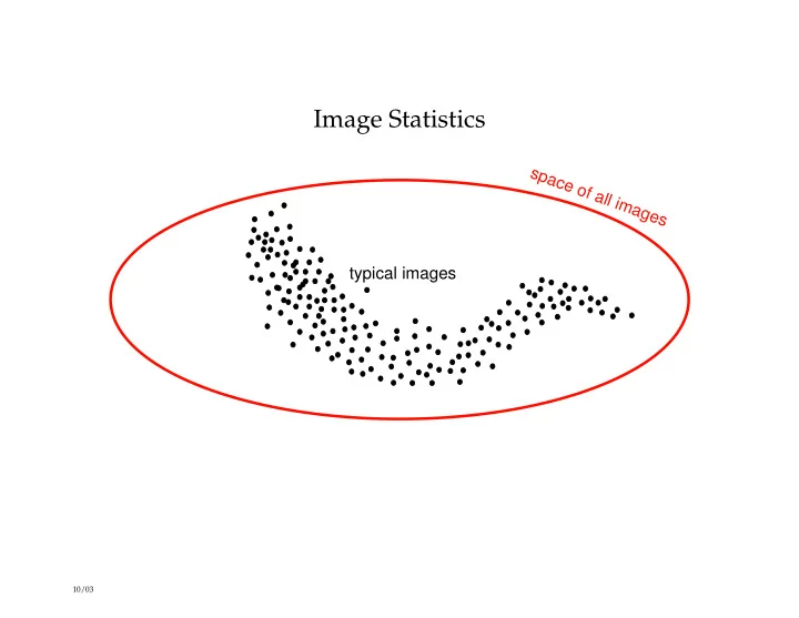
Image Statistics space of all images typical images 10/03 Image - - PowerPoint PPT Presentation

Image Statistics

space of all images typical images

10/03

Image Statistical Model Applications

Image Processing / Graphics:

• Noise removal: How easily can we detect (and remove) artifacts or

distortions?

• Compression: how compactly can we represent an image?
• Synthesis: can we make realistic-looking synthetic images?

Theoretical Neurobiology:

• Do sensory neurons perform optimal decomposition of images?
• If so, how does the system learn this decomposition?

10/03

Image Denoising

y = x + w, where w is Gaussian, white. y is an observed transform coefficient. Bayes least squares solution: ˆ x(y) = E(x|y) =

dx P(y|x) P(x) x dx P(y|x) P(x)

10/03

Pixel Statistics

50 100 150 200 250 1000 2000 3000 4000 5000 6000 7000 8000

Range: [0, 230] Dims: [512, 512] / 2

50 100 150 200 250 0.5 1 1.5 2 2.5 x 10

Range: [0, 253] Dims: [512, 512] / 2

50 100 150 200 250 300 0.5 1 1.5 2 2.5 3 3.5 x 10

10/03

Principal Component Analysis (PCA)

Find linear transform (specifically, rotation and axis re-scaling) that trans- form the covariance matrix to the identity.

• 20

20

• 20

20 4

• 4

4

• 4

20

• 20

20

• 20

a. b. c.

Well-known eigenvalue/eigenvector solution Assuming translation-invariance (stationarity), Fourier transform suf- fices Assuming scale-invariance, spectrum must fall as 1/f α

10/03

Image Spectra

10 10

1

10

2

10

3

10 10

1

10

2

10

3

10

4

10

5

10

6

Spatial−frequency (cycles/image) Power

Empirically, power spectrum of natural images falls as 1/f α, α ∼ 2.

[Field ’87, Ruderman & Bialek ’94, etc]

10/03

Model I: Fourier+Gaussian

Basis set: Image: Coefficient density:

• 10/03

Denoising I (Fourier/Gaussian)

Bayes Least Squares solution is linear (Wiener filter): E(xf|yf) = σ2

f

σ2

f + σ2 w

yf

5 10 15 20 signal noise −3 −2 −1 1 2 3 0.5 1 Wiener filter frequency

10/03

Denoising I

10/03

PCA is Insufficient

a. b.

left: 1/f Gaussian noise. right: whitened natural image. [after Field,

’87]

10/03

Bandpass Filters Reveal non-Gaussian Behaviors

−500 500 10

−4

10

−2

10

Filter Response Probability

Response histogram Gaussian density

Marginal densities of bandpass filtered images are non-Gaussian (and thus have higher entropy than a Gaussian of the same variance)

[Field ’87; Mallat ’89; Simoncelli etal. ’90; Zetzsche ’90]

10/03

PCA on Linear Combination of non-Gaussian Sources

−0.4 −0.2 0.2 0.4 −0.4 −0.3 −0.2 −0.1 0.1 0.2 0.3 0.4

Linear Mixture

−0.4 −0.2 0.2 0.4 −0.4 −0.3 −0.2 −0.1 0.1 0.2 0.3 0.4

After PCA Rotation

−4 −2 2 4 −4 −3 −2 −1 1 2 3 4

After Whitening

2nd-order whitening does not necessarily recover independent sources! Need an additional rotation matrix...

10/03

Independent Component Analysis (ICA)

Seek linear transform that maximizes statistical independence of trans- form coefficients. Many algorithms have been developed.

10/03

Fourth-order ICA (Cardoso ’89)

Diagonalize covariance matrix maximizes coefficient kurtosis (4th mo- ment divided by squared variance).

• 1. Rotate to PCA (2nd-order eigenvector) axes
• 2. Whiten (scale axes by inverse of corresponding eigenvalue)
• 3. Rotate to axes given by eigenvectors of:

E

• |

x|2 x · xT

• Recovers independent components,
• assuming linear mixture of independent sources
• assuming components have unique kurtoses
• up to axis re-ordering and re-scaling

10/03

ICA on Photographic Images

Linear operators with maximally independent (or maximally non-Gaussian) responses are oriented bandpass filters

[Bell/Sejnowski ’97; Olshausen/Field ’96]

10/03

Sample Kurtosis vs. Filter Bandwidth

0.5 1 1.5 2 2.5 3 4 6 8 10 12 14 16 Filter Bandwidth (octaves) Sample Kurtosis

For most images, maximum is near one octave [after Field, 1987].

10/03

Model II: ”Wavelet” + nonGaussian

Basis set: Image: Coefficient density:

• Need a basis of bandpass oriented filters (our next topic..)
• Need a model for the marginal densities

10/03

Example Marginals

Boats Lena Toys Goldhill

−100 −50 50 100 −100 −50 50 100 −100 −50 50 100 −100 −50 50 100

p = 0.62 p = 0.56 p = 0.52 p = 0.60 ∆H = 0.014 ∆H = 0.013 ∆H = 0.021 ∆H = 0.0019

• Coefficient densities well fit by generalized Laplacians

[Mallat 1989; Simoncelli/Adelson 1996]:

f(c) ∝ e−|c/s|p, p ∈ [0.5, 0.8].

• Non-Gaussianity due to both image content and choice of basis.

10/03

MAP estimator

p = 0.5 p = 1.0 p = 2.0 MAP estimators for generalized Gaussian coefficient prior with three different exponents. Dashed line is the identity function.

10/03

BLS estimator

p = 0.5 p = 1.0 p = 2.0

10/03

BLS estimator error

0.5 1 1.5 2 0.45 0.5 0.55 0.6 0.65 0.7 0.75 p Estimate variance / Noise variance

Error of BLS estimates as a function of the generalized Gaussian expo- nent.

10/03

Denoising system

Forward Transform Inverse Transform c0 c1 ck Estimators c0

^

c1

^

ck

^

Noisy Image

10/03

Denoising Simulation: Face

noisy (4.8) I-linear (10.61) II-marginal (11.98) III-GSM nbd: 5 × 5 + p (13.60)

• Semi-blind (all parameters estimated except for σw).
• SNR values shown in parentheses, log10(var(im)/var(err))

10/03