Image gradients and edges Tues Jan 24, 2017 Kristen Grauman - PDF document

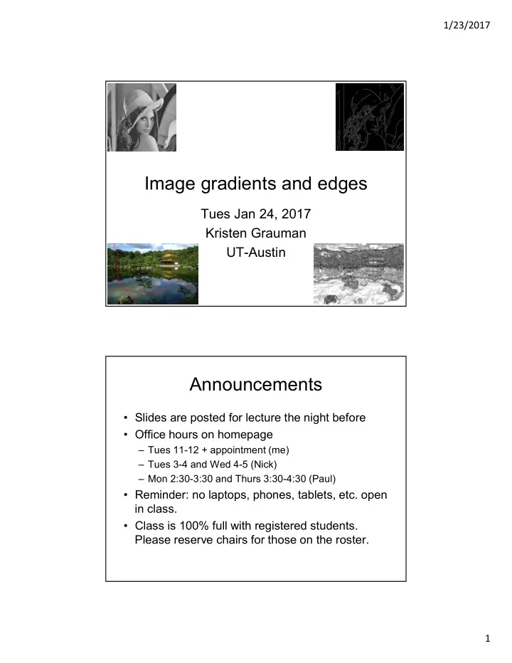
1/23/2017 Image gradients and edges Tues Jan 24, 2017 Kristen Grauman UT-Austin Announcements • Slides are posted for lecture the night before • Office hours on homepage – Tues 11-12 + appointment (me) – Tues 3-4 and Wed 4-5 (Nick) – Mon 2:30-3:30 and Thurs 3:30-4:30 (Paul) • Reminder: no laptops, phones, tablets, etc. open in class. • Class is 100% full with registered students. Please reserve chairs for those on the roster. 1

1/23/2017 Last time • Various models for image “noise” • Linear filters and convolution useful for – Image smoothing, removing noise • Box filter • Gaussian filter • Impact of scale / width of smoothing filter • Separable filters more efficient • Median filter: a non-linear filter, edge-preserving Image filtering • Compute a function of the local neighborhood at each pixel in the image – Function specified by a “filter” or mask saying how to combine values from neighbors. • Uses of filtering: – Enhance an image (denoise, resize, etc) – Extract information (texture, edges, etc) Today – Detect patterns (template matching) Adapted from Derek Hoiem 2

1/23/2017 Edge detection • Goal : map image from 2d array of pixels to a set of curves or line segments or contours. • Why? Figure from J. Shotton et al., PAMI 2007 • Main idea : look for strong gradients, post-process What causes an edge? Depth discontinuity: Reflectance change: object boundary appearance information, texture Cast shadows Change in surface orientation: shape 3

1/23/2017 Edges/gradients and invariance Derivatives and edges An edge is a place of rapid change in the image intensity function. intensity function image (along horizontal scanline) first derivative edges correspond to extrema of derivative Source: L. Lazebnik 4

1/23/2017 Derivatives with convolution For 2D function, f(x,y), the partial derivative is:     f ( x , y ) f ( x , y ) f ( x , y )  lim   x   0 For discrete data, we can approximate using finite differences:    f ( x , y ) f ( x 1 , y ) f ( x , y )   x 1 To implement above as convolution, what would be the associated filter? Partial derivatives of an image   f ( x , y ) f ( x , y )   x y ? -1 1 -1 1 or 1 -1 Which shows changes with respect to x? (showing filters for correlation) 5

1/23/2017 Image gradient The gradient of an image: The gradient points in the direction of most rapid change in intensity The gradient direction (orientation of edge normal) is given by: The edge strength is given by the gradient magnitude Slide credit Steve Seitz Effects of noise Consider a single row or column of the image • Plotting intensity as a function of position gives a signal Where is the edge? Slide credit Steve Seitz 6

1/23/2017 Solution: smooth first Where is the edge? Look for peaks in Derivative theorem of convolution Differentiation property of convolution. Slide credit Steve Seitz 7

1/23/2017 Derivative of Gaussian filters      ( I g ) h I ( g h )   0.0030 0.0133 0.0219 0.0133 0.0030   0.0133 0.0596 0.0983 0.0596 0.0133  1  1 0.0219 0.0983 0.1621 0.0983 0.0219 0.0133 0.0596 0.0983 0.0596 0.0133 0.0030 0.0133 0.0219 0.0133 0.0030 Derivative of Gaussian filters y -direction x -direction Source: L. Lazebnik 8

1/23/2017 Laplacian of Gaussian Consider Laplacian of Gaussian operator Where is the edge? Zero-crossings of bottom graph Slide credit: Steve Seitz 2D edge detection filters Laplacian of Gaussian Gaussian derivative of Gaussian • is the Laplacian operator: Slide credit: Steve Seitz 9

1/23/2017 Smoothing with a Gaussian Recall: parameter σ is the “scale” / “width” / “spread” of the Gaussian kernel, and controls the amount of smoothing. … Effect of σ on derivatives σ = 1 pixel σ = 3 pixels The apparent structures differ depending on Gaussian’s scale parameter. Larger values: larger scale edges detected Smaller values: finer features detected 10

1/23/2017 So, what scale to choose? It depends what we’re looking for. Mask properties • Smoothing – Values positive – Sum to 1  constant regions same as input – Amount of smoothing proportional to mask size – Remove “high-frequency” components; “low-pass” filter • Derivatives – ___________ signs used to get high response in regions of high contrast – Sum to ___  no response in constant regions – High absolute value at points of high contrast 11

1/23/2017 Seam carving: main idea [Shai & Avidan, SIGGRAPH 2007] Seam carving: main idea Content-aware resizing Traditional resizing [Shai & Avidan, SIGGRAPH 2007] 12

1/23/2017 Seam carving: main idea Real image example 13

1/23/2017 Seam carving: main idea Content-aware resizing Intuition: • Preserve the most “interesting” content  Prefer to remove pixels with low gradient energy • To reduce or increase size in one dimension, remove irregularly shaped “seams”  Optimal solution via dynamic programming. Seam carving: main idea  Energy ( f ) • Want to remove seams where they won’t be very noticeable: – Measure “energy” as gradient magnitude • Choose seam based on minimum total energy path across image, subject to 8-connectedness. 14

1/23/2017 Seam carving: algorithm s 1 s 2 s 3 s 4 s 5  Energy ( f ) Let a vertical seam s consist of h positions that form an 8-connected path. h   Let the cost of a seam be: Cost ( s ) Energy ( f ( s )) i  i 1 Optimal seam minimizes this cost:  s * min Cost ( s ) s Compute it efficiently with dynamic programming. How to identify the minimum cost seam? • First, consider a greedy approach: 1 3 0 2 8 9 5 2 6 Energy matrix (gradient magnitude) 15

1/23/2017 Seam carving: algorithm • Compute the cumulative minimum energy for all possible connected seams at each entry (i,j) :          M ( i , j ) Energy ( i , j ) min M ( i 1 , j 1 ), M ( i 1 , j ), M ( i 1 , j 1 ) row i-1 j-1 j j+1 row i j Energy matrix M matrix: (gradient magnitude) cumulative min energy (for vertical seams) • Then, min value in last row of M indicates end of the minimal connected vertical seam. • Backtrack up from there, selecting min of 3 above in M . Example          M ( i , j ) Energy ( i , j ) min M ( i 1 , j 1 ), M ( i 1 , j ), M ( i 1 , j 1 ) 1 3 0 1 3 0 2 8 9 3 8 9 5 2 6 8 5 14 Energy matrix M matrix (gradient magnitude) (for vertical seams) 16

1/23/2017 Example          M ( i , j ) Energy ( i , j ) min M ( i 1 , j 1 ), M ( i 1 , j ), M ( i 1 , j 1 ) 1 3 0 1 3 0 2 8 9 3 8 9 5 2 6 8 5 14 Energy matrix M matrix (gradient magnitude) (for vertical seams) Real image example Energy Map Original Image Blue = low energy Red = high energy 17

1/23/2017 Real image example Other notes on seam carving • Analogous procedure for horizontal seams • Can also insert seams to increase size of image in either dimension – Duplicate optimal seam, averaged with neighbors • Other energy functions may be plugged in – E.g., color-based, interactive,… • Can use combination of vertical and horizontal seams 18

1/23/2017 Example results from prior classes Results from Eunho Yang Conventional resize Original image Seam carving result Results from Martin Becker 19

1/23/2017 Conventional resize Original image Seam carving result Results from Martin Becker Conventional resize (399 by 599) Original image (599 by 799) Seam carving (399 by 599) Results from Jay Hennig 20

1/23/2017 Removal of a marked object Results from Donghyuk Shin Removal of a marked object Results from Eunho Yang 21

1/23/2017 “Failure cases” with seam carving By Donghyuk Shin “Failure cases” with seam carving By Suyog Jain 22

1/23/2017 Gradients -> edges Primary edge detection steps: 1. Smoothing: suppress noise 2. Edge enhancement: filter for contrast 3. Edge localization Determine which local maxima from filter output are actually edges vs. noise • Threshold, Thin Thresholding • Choose a threshold value t • Set any pixels less than t to zero (off) • Set any pixels greater than or equal to t to one (on) 23

1/23/2017 Original image Gradient magnitude image 24

1/23/2017 Thresholding gradient with a lower threshold Thresholding gradient with a higher threshold 25

1/23/2017 Canny edge detector • Filter image with derivative of Gaussian • Find magnitude and orientation of gradient • Non-maximum suppression : – Thin wide “ridges” down to single pixel width • Linking and thresholding ( hysteresis ): – Define two thresholds: low and high – Use the high threshold to start edge curves and the low threshold to continue them • MATLAB: edge(image, ‘canny’); • >>help edge Source: D. Lowe, L. Fei-Fei The Canny edge detector original image (Lena) Slide credit: Steve Seitz 26

1/23/2017 The Canny edge detector norm of the gradient The Canny edge detector thresholding 27