Image-based Lighting (Part 2) T2 Computational Photography Derek - - PowerPoint PPT Presentation

10/16/14

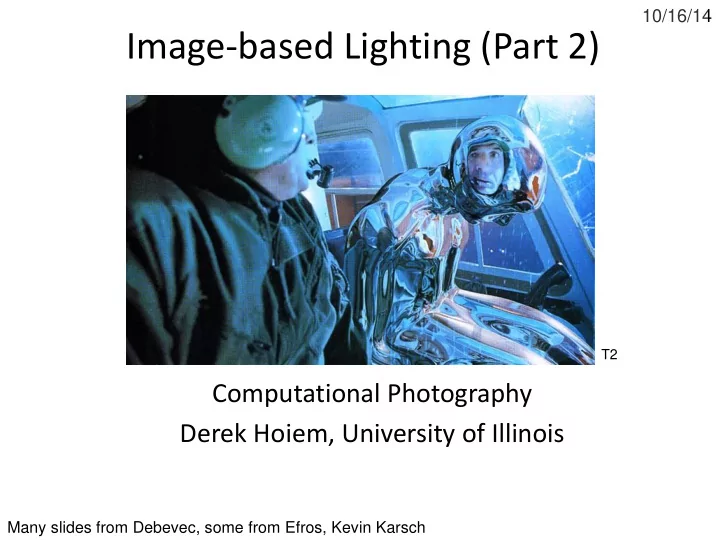
Image-based Lighting (Part 2)

Computational Photography Derek Hoiem, University of Illinois

Many slides from Debevec, some from Efros, Kevin Karsch

T2

Today

• Brief review of last class
• Show how to get an HDR image from several

LDR images, and how to display HDR

• Show how to insert fake objects into real

scenes using environment maps

How to render an object inserted into an image?

How to render an object inserted into an image? Traditional graphics way

• Manually model BRDFs of all room surfaces
• Manually model radiance of lights
• Do ray tracing to relight object, shadows, etc.

How to render an object inserted into an image? Image-based lighting

• Capture incoming light with a

“light probe”

• Model local scene
• Ray trace, but replace distant

scene with info from light probe

Debevec SIGGRAPH 1998

Key ideas for Image-based Lighting

• Environment maps: tell what light is entering

at each angle within some shell

+

Spherical Map Example

Key ideas for Image-based Lighting

• Light probes: a way of capturing environment

maps in real scenes

Mirrored Sphere

1) Compute normal of sphere from pixel position 2) Compute reflected ray direction from sphere normal 3) Convert to spherical coordinates (theta, phi) 4) Create equirectangular image

Mirror ball -> equirectangular

Mirror ball Equirectangular Normals Reflection vectors Phi/theta of reflection vecs Phi/theta equirectangular domain

Mirror ball -> equirectangular

One small snag

• How do we deal with light sources? Sun, lights,

etc?

– They are much, much brighter than the rest of the environment

• Use High Dynamic Range photography!

1 46 1907 15116 18

. . . . .

Relative Brightness

Key ideas for Image-based Lighting

• Capturing HDR images: needed so that light

probes capture full range of radiance

Problem: Dynamic Range

Long Exposure

10-6 106 10-6 106

Real world Picture

0 to 255

High dynamic range

Short Exposure

10-6 106 10-6 106

Real world Picture

High dynamic range

0 to 255

LDR->HDR by merging exposures

10-6 106

Real world

High dynamic range

0 to 255

Exposure 1 … Exposure 2 Exposure n

Ways to vary exposure

• Shutter Speed (*)
• F/stop (aperture, iris)
• Neutral Density (ND) Filters

Shutter Speed

Ranges: Canon EOS-1D X: 30 to 1/8,000 sec. ProCamera for iOS: ~1/10 to 1/2,000 sec. Pros:

• Directly varies the exposure
• Usually accurate and repeatable

Issues:

• Noise in long exposures

Recovering High Dynamic Range Radiance Maps from Photographs

Paul Debevec Jitendra Malik

August 1997 Computer Science Division University of California at Berkeley

The Approach

• Get pixel values Zij for image with shutter time Δtj

(ith pixel location, jth image)

• Exposure is irradiance integrated over time:
• Pixel values are non-linearly mapped Eij’s:
• Rewrite to form a (not so obvious) linear system:

Eij = Ri ×Dtj Zij = f (Eij)= f (Ri ×Dtj)

ln f -1(Zij) = ln(Ri)+ln(Dt j) g(Zij) = ln(Ri)+ln(Dt j)

The objective

Solve for radiance R and mapping g for each

• f 256 pixel values to minimize:

 

 

  

     

max min

Z Z z N i P j ij j i ij

z g z w Z g t R Z w

2 1 1 2

) ( ) ( ) ( ln ln ) ( 

give pixels near 0

• r 255 less weight

known shutter time for image j irradiance at particular pixel site is the same for each image exposure should smoothly increase as pixel intensity increases exposure, as a function of pixel value

Matlab Code

Matlab Code

function [g,lE]=gsolve(Z,B,l,w) n = 256; A = zeros(size(Z,1)*size(Z,2)+n+1,n+size(Z,1)); b = zeros(size(A,1),1); k = 1; %% Include the data-fitting equations for i=1:size(Z,1) for j=1:size(Z,2) wij = w(Z(i,j)+1); A(k,Z(i,j)+1) = wij; A(k,n+i) = -wij; b(k,1) = wij * B(i,j); k=k+1; end end A(k,129) = 1; %% Fix the curve by setting its middle value to 0 k=k+1; for i=1:n-2 %% Include the smoothness equations A(k,i)=l*w(i+1); A(k,i+1)=-2*l*w(i+1); A(k,i+2)=l*w(i+1); k=k+1; end x = A\b; %% Solve the system using pseudoinverse g = x(1:n); lE = x(n+1:size(x,1));

• 3
• 1 •

2 t = 1 sec

• 3
• 1 •

2 t = 1/16 sec

• 3
• 1
• 2

t = 4 sec

• 3
• 1 •

2 t = 1/64 sec

Illustration

Image series

• 3
• 1 •

2 t = 1/4 sec

Exposure = Radiance * t log Exposure = log Radiance  log t Pixel Value Z = f(Exposure)

Response Curve

ln Exposure

Assuming unit radiance

for each pixel

After adjusting radiances to

• btain a smooth response curve

Pixel value

3 1 2

ln Exposure Pixel value

Results: Digital Camera

Recovered response curve log Exposure Pixel value Kodak DCS460 1/30 to 30 sec

Reconstructed radiance map

Results: Color Film

• Kodak Gold ASA 100, PhotoCD

Recovered Response Curves

Red Green RGB Blue

How to display HDR?

Linearly scaled to display device

Global Operator (Reinhart et al)

world world display

L L L   1

Global Operator Results

Darkest 0.1% scaled to display device Reinhart Operator

Local operator

Acquiring the Light Probe

Assembling the Light Probe

Real-World HDR Lighting Environments

Lighting Environments from the Light Probe Image Gallery: http://www.debevec.org/Probes/ Funston Beach Uffizi Gallery Eucalyptus Grove Grace Cathedral

Illumination Results

Rendered with Greg Larson’s

Comparison: Radiance map versus single image

HDR LDR

CG Objects Illuminated by a Traditional CG Light Source

Illuminating Objects using Measurements of Real Light

Object Light

http://radsite.lbl.gov/radiance/ Environment assigned “glow” material property in Greg Ward’s RADIANCE system.

Paul Debevec. A Tutorial on Image-Based Lighting. IEEE Computer Graphics and Applications, Jan/Feb 2002.

Rendering with Natural Light

SIGGRAPH 98 Electronic Theater

Movie

• http://www.youtube.com/watch?v=EHBgkeXH9lU

Illuminating a Small Scene

We can now illuminate synthetic objects with real light.

• Environment map
• Light probe
• HDR
• Ray tracing

How do we add synthetic objects to a real scene?

Real Scene Example

Goal: place synthetic objects on table

real scene

Modeling the Scene

light-based model

Light Probe / Calibration Grid

real scene

Modeling the Scene

synthetic objects light-based model local scene

Differential Rendering

Local scene w/o objects, illuminated by model

The Lighting Computation

synthetic objects (known BRDF) distant scene (light-based, unknown BRDF) local scene (estimated BRDF)

Rendering into the Scene

Background Plate

Rendering into the Scene

Objects and Local Scene matched to Scene

Differential Rendering Difference in local scene

• =

Differential Rendering

Final Result

IMAGE-BASED LIGHTING IN FIAT LUX

Paul Debevec, Tim Hawkins, Westley Sarokin, H. P. Duiker, Christine Cheng, Tal Garfinkel, Jenny Huang SIGGRAPH 99 Electronic Theater

Fiat Lux

• http://ict.debevec.org/~debevec/FiatLux/movie/
• http://ict.debevec.org/~debevec/FiatLux/technology/

HDR Image Series

2 sec 1/4 sec 1/30 sec 1/250 sec 1/2000 sec 1/8000 sec

Assembled Panorama

Light Probe Images

Capturing a Spatially-Varying Lighting Environment

What if we don’t have a light probe?

Insert Relit Face Zoom in on eye Environment map from eye http://www1.cs.columbia.edu/CAVE/projects/world_eye/ -- Nishino Nayar 2004

Environment Map from an Eye

Can Tell What You are Looking At

Eye Image: Computed Retinal Image:

Video

Summary

• Real scenes have complex

geometries and materials that are difficult to model

• We can use an environment map,

captured with a light probe, as a replacement for distance lighting

• We can get an HDR image by

combining bracketed shots

• We can relight objects at that

position using the environment map