Image Analysis The topics of this lecture are Segmentation - PowerPoint PPT Presentation

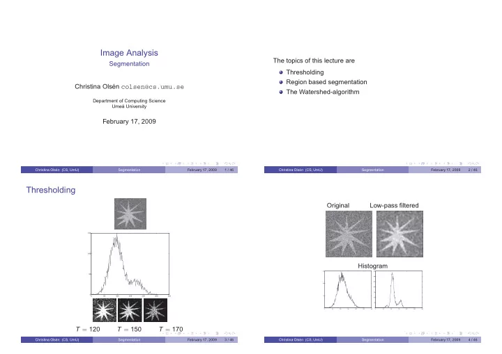
Image Analysis The topics of this lecture are Segmentation Thresholding Region based segmentation Christina Olsén colsen@cs.umu.se The Watershed-algorithm Department of Computing Science Umeå University February 17, 2009 Christina Olsén (CS, UmU) Segmentation February 17, 2009 1 / 46 Christina Olsén (CS, UmU) Segmentation February 17, 2009 2 / 46 Thresholding Original Low-pass filtered 150 100 Histogram 150 350 50 300 250 100 200 150 0 0 50 100 150 200 250 300 50 100 50 0 0 0 50 100 150 200 250 300 0 50 100 150 200 250 300 T = 120 T = 150 T = 170 Christina Olsén (CS, UmU) Segmentation February 17, 2009 3 / 46 Christina Olsén (CS, UmU) Segmentation February 17, 2009 4 / 46

We do not live in a perfect world Due to noise, uneven lightning and uneven intensity of the object Suppose that there is one object present in the image and that it and the background we can not assume that all pixels are of two different intensity has a specific intensity µ 1 Suppose that this intensity is different from the intensity µ 2 of the Suppose that there is one object and the background present in the image background We say that the intensity of the object is given by the probability In a perfect world it is sufficient to say that: Pixels with intensity value µ 1 constitute the object and pixels with density function p 1 ( z ) and the intensity of the background is given by p 2 ( z ) intensity µ 2 constitute the background The a-priori probability for a pixel to belong to the object is P 1 and to the background P 2 Since we only have one object it must hold that P 1 + P 2 = 1 Christina Olsén (CS, UmU) Segmentation February 17, 2009 5 / 46 Christina Olsén (CS, UmU) Segmentation February 17, 2009 6 / 46 Obviously we want to find the T that yields the lowest error We say that we have a mixture model That is the T that minimizes p ( z ) = P 1 p 1 ( z ) + P 2 p 2 ( z ) E ( T ) = P 2 E 1 ( T ) + P 1 E 2 ( T ) The histogram of the image is an estimate of this model To find this T we solve dE dT = 0 and obtains: Suppose that we establish a single threshold T and say that pixels with intensity higher than T belongs to the object and P 1 p 1 ( T ) = P 2 p 2 ( T ) pixels with intensity lower than T belongs to the background The error of using this threshold is The observable error against the histogram h ( z ) is n E ( T ) = P 2 E 1 ( T ) + P 1 E 2 ( T ) e = 1 � ( p ( z i ) − h ( z i )) 2 n where i = 1 � T E 1 ( T ) = p 2 ( z ) dz Without doing any assumptions, it is very hard to minimize e −∞ This can be handled in two ways and ◮ By assuming that we know the form of the distributions p 1 ( z ) and � ∞ E 2 ( T ) = p 1 ( z ) dz p 2 ( z ) and solve for T analytically ◮ Or we can solve for T by iterative numerical methods T Christina Olsén (CS, UmU) Segmentation February 17, 2009 7 / 46 Christina Olsén (CS, UmU) Segmentation February 17, 2009 8 / 46

Analytical Analytical We assume that p 1 and p 2 are normal distributed we obtain (for p 1 ( z ) ) The optimal T is the solution to AT 2 + BT + C = 0 1 e − ( z − µ 1 ) 2 / 2 σ 2 √ p 1 ( z ) = 1 2 πσ 1 where where µ 1 and σ 2 1 are the expected value and variance for the distribution. σ 2 1 − σ 2 A = 2 We can now find the optimal T by solving 2 ( µ 1 σ 2 2 − µ 2 σ 2 B = 1 ) σ 2 1 µ 2 2 − σ 2 2 µ 2 1 + 2 σ 2 1 σ 2 C = 2 ln ( σ 2 P 1 /σ 1 P 2 ) p 1 ( T ) P 1 = p 2 ( T ) P 2 analytically. Christina Olsén (CS, UmU) Segmentation February 17, 2009 9 / 46 Christina Olsén (CS, UmU) Segmentation February 17, 2009 10 / 46 −3 −3 x 10 x 10 3.5 4 object: µ 1 :160, σ 1 : 10 P 1 :0.3 3.5 3 object: µ 1 :150, σ 1 : 10 P 1 :0.3 3 2.5 2.5 2 background: µ 2 : 70, σ 2 : 40 P 2 :0.7 2 background: µ 2 : 90, σ 2 : 40 P 2 :0.7 1.5 1.5 1 1 T 1 :135 0.5 0.5 T 1 :140 T 2 :173 T 2 :192 0 0 0 50 100 150 200 250 300 0 50 100 150 200 250 300 Lowest error if object are pixelvalues 140 < I < 192: 3.58 % Lowest error if object are pixelvalues 135 < I < 173: 10.3 % Christina Olsén (CS, UmU) Segmentation February 17, 2009 11 / 46 Christina Olsén (CS, UmU) Segmentation February 17, 2009 12 / 46

Iterative Let i = 0 1 Calculate the center of mass of the histogram 2 The success of our analytical approach is dependent on � z h ( z ) · z T i = ◮ How well we can estimate the types of distributions � z h ( z ) ◮ How well we can estimate the parameters that control the distributions Calculate 3 ◮ How hard it is to solve the equations involved µ 0 ( T i ) = µ [ h ( z ) | z < T i ] Most of the times we must use iterative solutions and µ 1 ( T i ) = µ [ h ( z ) | z ≥ T i ] Let 4 T i + 1 = µ 0 ( T i ) + µ 1 ( T i ) 2 If | T i − T i + 1 | < ǫ then end, otherwise let i = i + 1 and go to 3. 5 Christina Olsén (CS, UmU) Segmentation February 17, 2009 13 / 46 Christina Olsén (CS, UmU) Segmentation February 17, 2009 14 / 46 Histogram 150 100 50 0 0 50 100 150 200 250 300 Threshold T = 128 Christina Olsén (CS, UmU) Segmentation February 17, 2009 15 / 46 Christina Olsén (CS, UmU) Segmentation February 17, 2009 16 / 46

Histogram 140 120 100 80 60 40 20 0 0 50 100 150 200 250 300 Threshold T = 120 Christina Olsén (CS, UmU) Segmentation February 17, 2009 17 / 46 Christina Olsén (CS, UmU) Segmentation February 17, 2009 18 / 46 Histogram Let i = 0 1 140 Let T i be some suitable value. 2 120 Define 3 100 p i 0 ( z ) = [ h ( z ) | z < T i ] 80 60 and p i 1 ( z ) = [ h ( z ) | z ≥ T i ] 40 20 Calculate P i 0 , µ i 0 and σ i 0 for p i 0 ( z ) and p i 4 1 0 0 50 100 150 200 250 300 Calculate a T i + 1 ∈ ( 0 , L max ) from 5 AT 2 i + 1 + BT i + 1 + C = 0 where A = σ 2 0 − σ 2 1 , B = 2 ( µ 0 σ 2 1 − µ 1 σ 2 0 ) and C = σ 2 0 µ 2 1 − σ 2 1 µ 2 0 + 2 σ 2 0 σ 2 1 ln ( σ 2 P 1 /σ 1 P 2 ) If | T i − T i + 1 | < ǫ then end, otherwise let i = i + 1 and go to 3. 6 Christina Olsén (CS, UmU) Segmentation February 17, 2009 19 / 46 Christina Olsén (CS, UmU) Segmentation February 17, 2009 20 / 46

Histogram 140 120 100 80 60 40 20 0 0 50 100 150 200 250 300 Threshold T = 148 Christina Olsén (CS, UmU) Segmentation February 17, 2009 21 / 46 Christina Olsén (CS, UmU) Segmentation February 17, 2009 22 / 46 Otsu The aim with thresholding is to divide the histogram (i.e. the intensity values in the image) into two parts. If we choose the approach to minimize the variance of the object and background pixels respectively it has been noticed that we often obtain thresholds that are close to optimal. Threshold T = 138 Christina Olsén (CS, UmU) Segmentation February 17, 2009 23 / 46 Christina Olsén (CS, UmU) Segmentation February 17, 2009 24 / 46

To calculate σ 2 within for each T can be rather costly By using the relationship The total variance within objects for a given threshold T is defined as between = σ 2 − σ 2 σ 2 within = n B ( T )( µ B ( T ) − µ ) 2 + n O ( T )( µ O ( T ) − µ ) 2 σ 2 within ( T ) = n B ( T ) σ 2 B ( T ) + n O ( T ) σ 2 O ( T ) = n B ( T ) n O ( T )( µ B ( T ) − µ O ( T )) 2 n B = � T − 1 i = 0 p ( i ) , n O = � L − 1 i = T p ( i ) σ 2 B and σ 2 O is the variance for background and object respectively. We can find the T that maximizes σ 2 The aim is to choose the T that minimizes σ 2 between within It can also be shown that the values can be updated iteratively This method is called Otsu’s method and is implemented in MatLabs greythresh command Christina Olsén (CS, UmU) Segmentation February 17, 2009 25 / 46 Christina Olsén (CS, UmU) Segmentation February 17, 2009 26 / 46 Otsus Method Thresholding T = 125 Christina Olsén (CS, UmU) Segmentation February 17, 2009 27 / 46 Christina Olsén (CS, UmU) Segmentation February 17, 2009 28 / 46

Region based methods Region growing The segmentation of an image involves dividing it into regions R 1 , R 2 , . . . , R n for which holds: Let i = 0 1 � i R i = R 1 choose a start region r i 2 R i is a connected component, ∀ i � r i . Where p i are the neighbors r i that full fills 2 Define r i + 1 = p i 3 R i ∩ R j = ∅ ∀ i � = j 3 the predicate P ( p i ) P ( R i ) = TRUE , ∀ i 4 If p i = ∅ then end otherwise let i = i + 1 and goto 3. 4 P ( R i ∪ R j ) = FALSE , ∀ i � = j 5 P is a logical predicate defined on all points that belong to a region Christina Olsén (CS, UmU) Segmentation February 17, 2009 29 / 46 Christina Olsén (CS, UmU) Segmentation February 17, 2009 30 / 46 Quad-tree The previous methods is based on choice of start region Region−växning Δ T =10% Region−växning Δ T =5% Original One way round this is to start from the top-region R (i.e. the entire image) and divide it The division is carried out repeatedly for all regions not meeting a criteria P . The division is carried on recursively until all regions have size 1 or they all meet the criteria P . The sub-division is made easier if the image has side length of the form N = 2 n When the division is carried out all regions that fulfill P is merged to one Christina Olsén (CS, UmU) Segmentation February 17, 2009 31 / 46 Christina Olsén (CS, UmU) Segmentation February 17, 2009 32 / 46