Image alignment What to do if we want to compare the appearance of - PowerPoint PPT Presentation

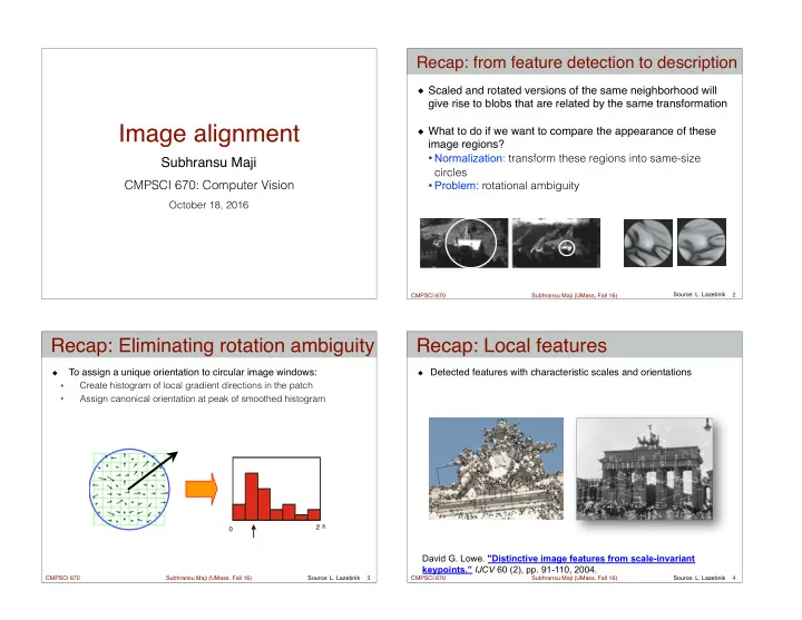
Recap: from feature detection to description Scaled and rotated versions of the same neighborhood will give rise to blobs that are related by the same transformation Image alignment What to do if we want to compare the appearance of these image regions? • Normalization : transform these regions into same-size Subhransu Maji circles • Problem: rotational ambiguity CMPSCI 670: Computer Vision October 18, 2016 Source: L. Lazebnik 2 CMPSCI 670 Subhransu Maji (UMass, Fall 16) Recap: Eliminating rotation ambiguity Recap: Local features To assign a unique orientation to circular image windows: Detected features with characteristic scales and orientations ‣ Create histogram of local gradient directions in the patch ‣ Assign canonical orientation at peak of smoothed histogram 2 π 0 David G. Lowe. "Distinctive image features from scale-invariant keypoints.” IJCV 60 (2), pp. 91-110, 2004. Source: L. Lazebnik Source: L. Lazebnik CMPSCI 670 Subhransu Maji (UMass, Fall 16) 3 CMPSCI 670 Subhransu Maji (UMass, Fall 16) 4


 
 
 
 
 
 
 
 
 
 
 Feature descriptors Feature descriptors Find regions and compare their feature descriptors Simplest descriptor: vector of raw intensity values How to compare two such vectors? ‣ Sum of squared differences (SSD) — this is a distance measure 
 2 SSD( u, v ) ( u v ) ∑ = − i i i ➡ Not invariant to intensity change 
 ‣ Normalized correlation — this is a similarity measure 
 ( u u )( v v ) ∑ ( u u ) ( v v ) − − − − i i ( u, v ) i ρ = ⋅ = || u u || || v v || − − & # & # 2 2 ( u u ) ( v v ) $ ∑ ! $ ∑ ! − − j j $ ! $ ! % " % " j j ➡ Invariant to affine (translation + scaling) intensity change 5 6 CMPSCI 670 Subhransu Maji (UMass, Fall 16) CMPSCI 670 Subhransu Maji (UMass, Fall 16) Problem with intensity vectors Feature descriptors: SIFT Descriptor computation: Small deformations can affect the matching score a lot 
 ‣ Divide patch into 4x4 sub-patches ‣ Compute histogram of gradient orientations (8 reference angles) inside each sub-patch ‣ Resulting descriptor: 4x4x8 = 128 dimensions David G. Lowe. "Distinctive image features from scale-invariant keypoints.” IJCV 60 (2), pp. 91-110, 2004. CMPSCI 670 Subhransu Maji (UMass, Fall 16) 7 CMPSCI 670 Subhransu Maji (UMass, Fall 16) 8

Problem: Ambiguous putative matches Feature descriptors: SIFT Descriptor computation: ‣ Divide patch into 4x4 sub-patches ‣ Compute histogram of gradient orientations (8 reference angles) inside each sub-patch ‣ Resulting descriptor: 4x4x8 = 128 dimensions 
 Advantage over raw vectors of pixel values ‣ Gradients less sensitive to illumination change ‣ Pooling of gradients over the sub-patches achieves robustness to small shifts, but still preserves some spatial information More on image representations later David G. Lowe. "Distinctive image features from scale-invariant keypoints.” IJCV 60 (2), pp. 91-110, 2004. Source: Y. Furukawa 9 10 CMPSCI 670 Subhransu Maji (UMass, Fall 16) CMPSCI 670 Subhransu Maji (UMass, Fall 16) Rejection of unreliable matches A framework for alignment How can we tell which putative matches are more reliable? Matching local features Heuristic: compare distance of nearest neighbor to that of second ‣ Local information used, can contain outliers nearest neighbor ‣ But hopefully enough of these matches are good ‣ Ratio of closest distance to second-closest distance will be high 
 for features that are not distinctive Threshold of 0.8 provides good separation David G. Lowe. "Distinctive image features from scale-invariant keypoints.” IJCV 60 (2), pp. 91-110, 2004. CMPSCI 670 Subhransu Maji (UMass, Fall 16) 11 CMPSCI 670 Subhransu Maji (UMass, Fall 16) 12

A framework for alignment Families of transformation Matching local features ‣ Local information used, can contain outliers ‣ But hopefully enough of these matches are good Consensus building ‣ Aggregate the good matches and find a transformation that explains these matches 13 14 CMPSCI 670 Subhransu Maji (UMass, Fall 16) CMPSCI 670 Subhransu Maji (UMass, Fall 16) How do we move pixels? Points in 2D Think about moving coordinates, not pixels. CMPSCI 670 Subhransu Maji (UMass, Fall 16) 15 CMPSCI 670 Subhransu Maji (UMass, Fall 16) 16

Translation Scaling 17 18 CMPSCI 670 Subhransu Maji (UMass, Fall 16) CMPSCI 670 Subhransu Maji (UMass, Fall 16) Rotation Shear CMPSCI 670 Subhransu Maji (UMass, Fall 16) 19 CMPSCI 670 Subhransu Maji (UMass, Fall 16) 20

Arbitrary linear transformation Families of linear transforms 21 22 CMPSCI 670 Subhransu Maji (UMass, Fall 16) CMPSCI 670 Subhransu Maji (UMass, Fall 16) Affine transformations Fitting an affine transformation Affine = linear + translation Assume we know the correspondences, how do we get the transformation? x → Mx + t Approximates viewpoint changes for roughly planar objects and ( x i y , ) roughly orthographic cameras i ( x i y , ) ! ! i Can be used to initialize fitting for more complex models x Mx t ! = + i i x m m x t ' & # & # & # & # i 1 2 i 1 Want to find M , t to minimize = + $ ! $ ! $ ! $ ! y m m y t ' n % " % " % " % " i 3 4 i 2 2 || x Mx t || ∑ # − − i i i 1 = CMPSCI 670 Subhransu Maji (UMass, Fall 16) 23 CMPSCI 670 Subhransu Maji (UMass, Fall 16) 24

Fitting an affine transformation Fitting an affine transformation Assume we know the correspondences, how do we get the Linear system with six unknowns transformation? Each match gives us two linearly independent equations: need at least three to solve for the transformation parameters ( x i y , ) i ( x i y , ) ! ! m i & # 1 $ ! ! m ! & # & # 2 $ ! $ ! $ ! x y 0 0 1 0 m x $ ! ' i i 3 i $ ! $ ! = $ ! 0 0 x y 0 1 m y $ ! $ ' ! $ ! i i 4 i $ ! $ ! m & # ! $ t ! ! 1 % " % " 1 $ ! $ ! ! m ! & # & # t $ ! 2 $ ! % " 2 $ ! $ ! x m m x t x y 0 0 1 0 m x ' $ ! ' & # & # & # & # 3 i 1 2 i 1 $ i i ! $ i ! = = + $ ! $ ! $ ! $ ! $ ! 0 0 x y 0 1 m y y m m y t $ ! $ ' ! ' % " % " % " % " $ ! i i 4 i i 3 4 i 2 $ ! $ ! ! $ t ! ! % " % " 1 $ ! t $ ! % " 2 25 26 CMPSCI 670 Subhransu Maji (UMass, Fall 16) CMPSCI 670 Subhransu Maji (UMass, Fall 16) A framework for alignment RANSAC Matching local features Ran dom Sa mple C onsensus ‣ Local information used, can contain outliers Choose a small subset of points uniformly at random ‣ But hopefully enough of these matches are good Fit a model to that subset Consensus building Find all remaining points that are “close” to the model and ‣ Aggregate the good matches and find a transformation that reject the rest as outliers explains these matches Do this many times and choose the best model For rigid transformation we can estimate the parameters of the transformation, e.g., rotation angle, scaling, translation, etc, from putative correspondence matches Lets see how RANSAC works for a simple example. M. A. Fischler, R. C. Bolles. Random Sample Consensus: A Paradigm for Model Fitting with Applications to Image Analysis and Automated Cartography. Comm. of the ACM, Vol 24, pp 381-395, 1981. CMPSCI 670 Subhransu Maji (UMass, Fall 16) 27 CMPSCI 670 Subhransu Maji (UMass, Fall 16) 28

RANSAC for line fitting example RANSAC for line fitting example X ( ax i + b − y i ) 2 min a,b i Least-squares fit Source: R. Raguram Source: R. Raguram 29 30 CMPSCI 670 Subhransu Maji (UMass, Fall 16) CMPSCI 670 Subhransu Maji (UMass, Fall 16) RANSAC for line fitting example RANSAC for line fitting example 1. Randomly select 1. Randomly select minimal subset of minimal subset of points points 2. Hypothesize a model Source: R. Raguram Source: R. Raguram CMPSCI 670 Subhransu Maji (UMass, Fall 16) 31 CMPSCI 670 Subhransu Maji (UMass, Fall 16) 32

RANSAC for line fitting example RANSAC for line fitting example 1. Randomly select 1. Randomly select minimal subset of minimal subset of points points 2. Hypothesize a 2. Hypothesize a model model 3. Compute error 3. Compute error function function 4. Select points consistent with model Source: R. Raguram Source: R. Raguram 33 34 CMPSCI 670 Subhransu Maji (UMass, Fall 16) CMPSCI 670 Subhransu Maji (UMass, Fall 16) RANSAC for line fitting example RANSAC for line fitting example 1. Randomly select 1. Randomly select minimal subset of minimal subset of points points 2. Hypothesize a 2. Hypothesize a model model 3. Compute error 3. Compute error function function 4. Select points 4. Select points consistent with consistent with model model 5. Repeat hypothesize- 5. Repeat hypothesize- and-verify loop and-verify loop Source: R. Raguram Source: R. Raguram CMPSCI 670 Subhransu Maji (UMass, Fall 16) 35 CMPSCI 670 Subhransu Maji (UMass, Fall 16) 36