
University of British Columbia CPSC 314 Computer Graphics Jan-Apr 2010 Tamara Munzner http://www.ugrad.cs.ubc.ca/~cs314/Vjan2010
Lighting/Shading IV, Advanced Rendering I Week 7, Fri Mar 5
2
News
- midterm is Monday, be on time!
- HW2 solutions out
3
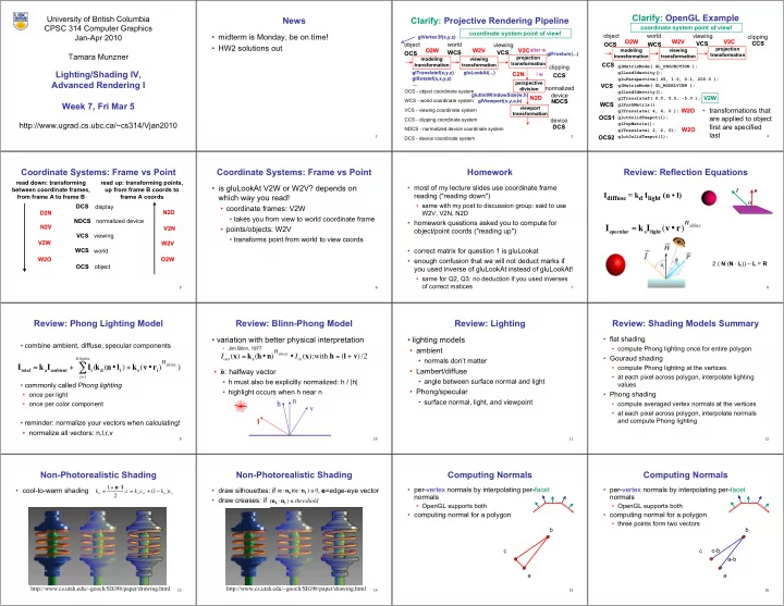
Clarify: Projective Rendering Pipeline
OCS - object coordinate system WCS - world coordinate system VCS - viewing coordinate system CCS - clipping coordinate system NDCS - normalized device coordinate system DCS - device coordinate system
OCS OCS WCS WCS VCS VCS CCS CCS NDCS NDCS DCS DCS
modeling modeling transformation transformation viewing viewing transformation transformation projection projection transformation transformation viewport viewport transformation transformation alter w alter w / w / w
- bject
world viewing device normalized device clipping
perspective perspective division division glVertex3f(x,y,z) glVertex3f(x,y,z) glTranslatef glTranslatef(x,y,z) (x,y,z) glRotatef glRotatef(a,x,y,z) (a,x,y,z) .... .... gluLookAt gluLookAt(...) (...) glFrustum glFrustum(...) (...) glutInitWindowSize glutInitWindowSize(w,h) (w,h) glViewport glViewport(x,y,a,b) (x,y,a,b)
O2W O2W W2V W2V V2C V2C N2D N2D C2N C2N coordinate system point of view!
4
Clarify: OpenGL Example
glMatrixMode( GL_PROJECTION ); glLoadIdentity(); gluPerspective( 45, 1.0, 0.1, 200.0 ); glMatrixMode( GL_MODELVIEW ); glLoadIdentity(); glTranslatef( 0.0, 0.0, -5.0 ); glPushMatrix() glTranslate( 4, 4, 0 ); glutSolidTeapot(1); glPopMatrix(); glTranslate( 2, 2, 0); glutSolidTeapot(1);
OCS2 OCS2 O2W O2W VCS VCS
modeling modeling transformation transformation viewing viewing transformation transformation projection projection transformation transformation
- bject
world viewing W2V W2V V2C V2C WCS WCS
- transformations that
are applied to object first are specified last
OCS1 OCS1 WCS WCS VCS VCS W2O W2O W2O W2O CCS CCS clipping CCS CCS OCS OCS coordinate system point of view! V2W V2W
5
NDCS NDCS
- bject
world viewing OCS OCS WCS WCS VCS VCS W2V W2V O2W O2W read down: transforming between coordinate frames, from frame A to frame B V2N V2N DCS DCS normalized device display read up: transforming points, up from frame B coords to frame A coords V2W V2W W2O W2O N2V N2V D2N D2N N2D N2D
Coordinate Systems: Frame vs Point
6
Coordinate Systems: Frame vs Point
- is gluLookAt V2W or W2V? depends on
which way you read!
- coordinate frames: V2W
- takes you from view to world coordinate frame
- points/objects: W2V
- transforms point from world to view coords
7
Homework
- most of my lecture slides use coordinate frame
reading ("reading down")
- same with my post to discussion group: said to use
W2V, V2N, N2D
- homework questions asked you to compute for
- bject/point coords ("reading up")
- correct matrix for question 1 is gluLookat
- enough confusion that we will not deduct marks if
you used inverse of gluLookAt instead of gluLookAt!
- same for Q2, Q3: no deduction if you used inverses
- f correct matices
8
Review: Reflection Equations
Idiffuse = kd Ilight (n • l)
n l θ 2 ( N (N · L)) – L = R
Ispecular = ksIlight(v•r)nshiny
9
Review: Phong Lighting Model
- combine ambient, diffuse, specular components
- commonly called Phong lighting
- once per light
- once per color component
- reminder: normalize your vectors when calculating!
- normalize all vectors: n,l,r,v
Itotal = kaIambient + Ii(
i=1 #lights
- kd(n•li) + ks(v•ri)nshiny )
10
Review: Blinn-Phong Model
- variation with better physical interpretation
- Jim Blinn, 1977
- h: halfway vector
- h must also be explicitly normalized: h / |h|
- highlight occurs when h near n
l l n n v v h h Iout(x) = ks(h•n)nshiny • Iin(x);with h = (l + v)/2
11
Review: Lighting
- lighting models
- ambient
- normals don’t matter
- Lambert/diffuse
- angle between surface normal and light
- Phong/specular
- surface normal, light, and viewpoint
12
Review: Shading Models Summary
- flat shading
- compute Phong lighting once for entire polygon
- Gouraud shading
- compute Phong lighting at the vertices
- at each pixel across polygon, interpolate lighting
values
- Phong shading
- compute averaged vertex normals at the vertices
- at each pixel across polygon, interpolate normals
and compute Phong lighting
13
Non-Photorealistic Shading
- cool-to-warm shading
http://www.cs.utah.edu/~gooch/SIG98/paper/drawing.html kw = 1+ n l 2 ,c = kwcw + (1 kw)cc
14
Non-Photorealistic Shading
- draw silhouettes: if , e=edge-eye vector
- draw creases: if
(e n0)(e n1) 0 http://www.cs.utah.edu/~gooch/SIG98/paper/drawing.html (n0 n1) threshold
15
Computing Normals
- per-vertex normals by interpolating per-facet
normals
- OpenGL supports both
- computing normal for a polygon
c b a
16
Computing Normals
- per-vertex normals by interpolating per-facet
normals
- OpenGL supports both
- computing normal for a polygon
- three points form two vectors
c b a c-b a-b