https://www.wolframalpha.com/input/?i=slope%20field - PowerPoint PPT Presentation

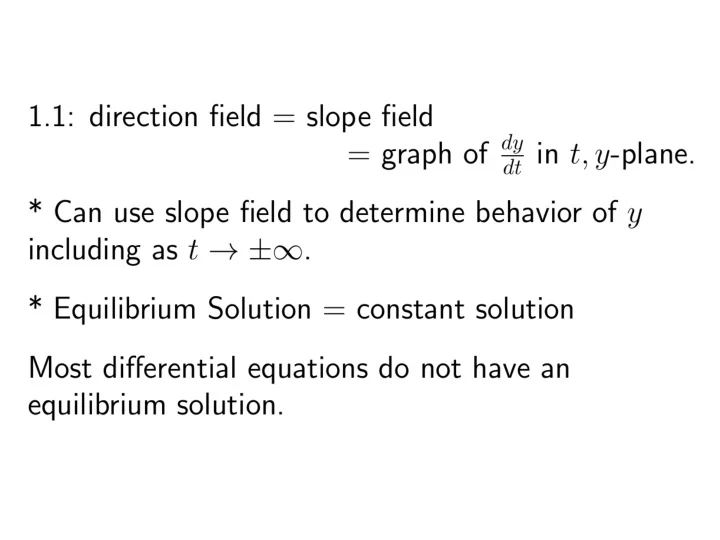
https://www.wolframalpha.com/input/?i=slope%20field

http://bcs.wiley.com/he-bcs/Books?action=resource &bcsId=2026&itemId=047143339X&resourceId=4140 Ch 2.2: Separable Equations In this section we examine a subclass of linear and nonlinear first order equations. Consider the first order equation dy = f ( x , y ) dx We can rewrite this in the form dy + = M ( x , y ) N ( x , y ) 0 dx For example, let M ( x , y ) = - f ( x , y ) and N ( x , y ) = 1. There may be other ways as well. In differential form, + = M ( x , y ) dx N ( x , y ) dy 0 If M is a function of x only and N is a function of y only, then + = M ( x ) dx N ( y ) dy 0 In this case, the equation is called separable .

http://bcs.wiley.com/he-bcs/Books?action=resource &bcsId=2026&itemId=047143339X&resourceId=4140 Example 1: Solving a Separable Equation Solve the following first order nonlinear equation: + 2 dy x 1 = y 2 − dx 1 Separating variables, and using calculus, we obtain ( ) ( ) − = + 2 2 y 1 dy x 1 dx ( ) ( ) ∫ ∫ − = + 2 2 y 1 dy x 1 dx 1 1 − = + + 3 3 y y x x C 3 3 3 − = 3 + + y 3 y x 3 x C The equation above defines the solution y implicitly. A graph showing the direction field and implicit plots of several integral curves for the differential equation is given above.

http://bcs.wiley.com/he-bcs/Books?action=resource&bcsId=2026&itemId=047143339X&resourceId=4140 Example 2: Implicit and Explicit Solutions (1 of 4) Solve the following first order nonlinear equation: + + 2 dy 3 x 4 x 2 = ( ) − dx 2 y 1 Separating variables and using calculus, we obtain ( ) ( ) − = + + 2 2 y 1 dy 3 x 4 x 2 dx ( ) ( ) ∫ ∫ − = + + 2 2 y 1 dy 3 x 4 x 2 dx − = + + + 2 3 2 y 2 y x 2 x 2 x C The equation above defines the solution y implicitly. An explicit expression for the solution can be found in this case: ( ) ± + + + + 3 2 ( ) 2 4 4 x 2 x 2 x C − − + + + = ⇒ = 2 3 2 y 2 y x 2 x 2 x C 0 y 2 = ± 3 + 2 + + y 1 x 2 x 2 x C

http://bcs.wiley.com/he-bcs/Books?action=resource &bcsId=2026&itemId=047143339X&resourceId=4140 Example 2: Initial Value Problem (2 of 4) Suppose we seek a solution satisfying y (0) = -1. Using the implicit expression of y , we obtain 2 − = 3 + 2 + + y 2 y x 2 x 2 x C − − − = ⇒ = 2 ( 1 ) 2 ( 1 ) C C 3 Thus the implicit equation defining y is − = + + + 2 3 2 y 2 y x 2 x 2 x 3 Using explicit expression of y , = ± + + + 3 2 y 1 x 2 x 2 x C − = ± ⇒ = 1 1 C C 4 It follows that = − + + + 3 2 y 1 x 2 x 2 x 4

http://bcs.wiley.com/he-bcs/Books?action=resource &bcsId=2026&itemId=047143339X&resourceId=4140 Example 2: Initial Condition y (0) = 3 (3 of 4) Note that if initial condition is y (0) = 3, then we choose the positive sign, instead of negative sign, on square root term: = + + + + 3 2 y 1 x 2 x 2 x 4

http://bcs.wiley.com/he-bcs/Books?action=resource &bcsId=2026&itemId=047143339X&resourceId=4140 Example 2: Domain (4 of 4) Thus the solutions to the initial value problem + + 2 dy 3 x 4 x 2 = = − , y ( 0 ) 1 ( ) − dx 2 y 1 are given by − = + + + 2 3 2 y 2 y x 2 x 2 x 3 (implicit) = − + + + 3 2 y 1 x 2 x 2 x 4 (explicit) From explicit representation of y , it follows that ) ( ) ( ) ( ) ( = − 2 + + + = − + 2 + y 1 x x 2 2 x 2 1 x 2 x 2 and hence domain of y is (-2, ∞ ). Note x = -2 yields y = 1, which makes denominator of dy / dx zero (vertical tangent). Conversely, domain of y can be estimated by locating vertical tangents on graph (useful for implicitly defined solutions).

http://bcs.wiley.com/he-bcs/Books?action=resource&bcsId=2026&itemId=047143339X&resourceId=4140 Example 3: Implicit Solution of Initial Value Problem (1 of 2) Consider the following initial value problem: y cos x ′ = = y , y ( 0 ) 1 + 3 1 3 y Separating variables and using calculus, we obtain + 3 1 3 y = dy cos xdx y   1 ∫ ∫   + = 2 3 y dy cos xdx   y   + 3 = + ln y y sin x C Using the initial condition, it follows that + = + 3 ln y y sin x 1

http://bcs.wiley.com/he-bcs/Books?action=resource &bcsId=2026&itemId=047143339X&resourceId=4140 Example 3: Graph of Solutions (2 of 2) Thus y cos x ′ = = ⇒ + 3 = + y , y ( 0 ) 1 ln y y sin x 1 + 3 1 3 y The graph of this solution (black), along with the graphs of the direction field and several integral curves (blue) for this differential equation, is given below.